Dynamic Programming

1. Basic Algorithmic Idea

It also solves problems by breaking down large problems into smaller ones, but it is specifically designed for cases where the subproblems are not independent.

Dynamic programming algorithms are often used to solve optimization problems. The decomposed substructures at each level usually overlap, meaning that the subproblems generated each time are not completely new; a subproblem may contain solutions to subproblems from the previous level. To improve computational efficiency, a table is generally used to record the solutions to subproblems so that they can be easily retrieved when combining upwards. Generally speaking, it can be designed according to the following steps:

1. Characterize the structure of an optimal solution;
2. Recursively define the value of an optimal solution;
3. Compute the value of an optimal solution in a bottom-up fashion;
4. Construct an optimal solution from the computed information.

Basic Elements of Dynamic Programming:

1. Optimal Substructure: A problem is said to have optimal substructure if an optimal solution to the problem contains within it optimal solutions to subproblems.
2. Overlapping Subproblems: When using a dynamic programming algorithm, the subproblems generated at each step are not entirely new; they may share common subproblems. By utilizing the table-recording method mentioned above, problems can generally be solved in polynomial time.
3. Memoization Method: This is a variation of the dynamic programming algorithm. Also using a table, the memoization method employs a top-down computational approach. It creates an entry for each subproblem, checks whether the subproblem has already been solved, uses the recorded value if it has, and otherwise computes and records it.

2. Algorithm Applications

2.1 Matrix Chain Multiplication

2.1.1 Problem Description

Given \(n\) matrices \(\{A_1, A_2, \dots, A_n\}\), where \(A_i\) and \(A_{i+1}\) are compatible for multiplication (\(i=1, 2, \dots, n-1\)). Find the matrix product \(A_1A_2\cdots A_n\).

Matrix multiplication is associative, so the order of multiplications can be altered. We use parenthesization to specify the order of multiplications in the matrix chain product.

For example, for the product of four matrices \(A_1A_2A_3A_4\), there are 5 possible parenthesizations: \[ \begin{gathered} (A_1(A_2(A_3A_4))),(A_1((A_2A_3)A_4)),((A_1A_2)(A_3A_4)),\\ ((A_1(A_2A_3))A_4),(((A_1A_2)A_3)A_4) \end{gathered} \] Due to the properties of matrix multiplication, different multiplication orders require different numbers of scalar multiplications. Let \(ra, ca\) and \(rb, cb\) denote the dimensions of matrices \(A\) and \(B\) respectively. The standard algorithm code to compute their matrix product is as follows:

1
2
3
4
5
6
7
8
9
10
11
12
13
14
15
16
17
18
19

void matrix_multiply(int **a, int **b, int ra, int ca, int rb, int cb)  //a,b表示表示矩阵
{
    if(ca != cb)
    {
        error("Unmultiplyable matrix!");
    }
    for(int i = 0; i < ra; i++)
    {
        for(int j = 0; j < cb; j++)
        {
            int sum = a[i][0]*b[0][j];
            for(int k = 1; k < ca; k++ )
            {
                sum += a[i][k]*b[k][j];
            }
            c[i][j] = sum;
        }
    }
}

2.1.2 Algorithm Design

For the matrix chain product \(A_iA_{i+1}\cdots A_j\), denote it as \(A[i:j]\). For a parenthesization \(((A_1\cdots A_k)(A_{k+1}\cdots A_n))\), the number of operations required is the cost of computing \(A[1:k]\) plus the cost of computing \(A[k+1:n]\), plus the cost of multiplying the two resulting matrices together.

Computing the Optimal Value:

Let \(m[i][j]\) be the minimum number of scalar multiplications needed to compute \(A[i:j]\) (\(1\leqslant i\leqslant j \leqslant n\)). The optimal solution to the original problem is the value of \(m[1][n]\). Assuming the optimal split occurs at \(k\) (\(i\leqslant k<j\)), \(m[i][j]\) can be recursively defined as:

\[ m[i][j]= \left\{ \begin{aligned} &0 &i=j \\ &\min_{i\leqslant k < j} \left \{ m[i][k]+m[k+1][j]+p_{i-1}p_{k}p_{j}\right\} &i<j \end{aligned} \right. \]

where \(p_i\) denotes the number of columns of matrix \(A_i\), and from the properties of matrix multiplication, \(p_{i-1}\) denotes the number of rows of matrix \(A_i\).

For each \(k\), there is a corresponding \(m[i][j]\). We establish another table \(s[i][j]\) to store the value of \(k\), so that after obtaining the optimal value \(m[i][j]\), the corresponding optimal solution can be reconstructed recursively from \(s[i][j]\). We compute the matrix \(m\) using the recurrence relation. The basic code is given below:

1
2
3
4
5
6
7
8
9
10
11
12
13
14
15
16
17
18
19
20
21
22
23
24
25
26

void matrix_chain(int *p, int n, int **m, int **s)
{
    for(int i = 1; i <= n; i++)
    {
        m[i][i] = 0;
    }

    for(int r = 2; r <= n; r++)
    {
        for(int i = 1; i <= n-r+1; i++)
        {
            int j = i+r-1;
            m[i][j] = m[i+1][j]+p[i-1]*p[i]*p[j];
            s[i][j] = i;
            for(int k = i+1; k < j; k++)
            {
                int t = m[i][k]+m[k+1][j]+p[i-1]*p[k]*p[j];
                if(t < m[i][j])
                {
                    m[i][j] = t;
                    s[i][j] = k;
                }
            }
        }
    }
}

Here is an example from the book Computer Algorithm Design and Analysis for better understanding. Suppose we need to compute the matrix chain product \(A_1A_2A_3A_4A_5A_6\). The dimensions are as follows:

The computation order and the corresponding \(m\) and \(s\) tables are as follows:

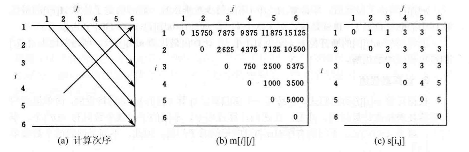
For example, when calculating \(m[1][3]\), the recurrence is:

During the computation, we find that the smaller value is achieved when \(k=1\), so \(s[1][3]=1\). After completing the computation of table \(m\), the optimal value \(m[1][n]\) is obtained.

Constructing the Optimal Solution:

The above method only computes the minimum number of operations, but does not provide the specific multiplication sequence. In fact, the data stored in table \(s\) contains the sequence information corresponding to each computation.

For example, the information recorded in \(s[1][n]\) indicates that the optimal way to compute \(A[1:n]\) is: \((A[1:s[1][n]])(A[s[1][n]+1:n])\). Similarly, the optimal parenthesization for the internal \(A[1:s[1][n]]\) is: \((A[1:s[1][s[1][n]]])(A[s[1][s[1][n]]+1:s[1][s[1][n]]])\). By continuing this recursion, the optimal computation order for \(A[1:n]\) can finally be determined. Below is the code implementation of this recursion:

1
2
3
4
5
6
7
8
9
10
11
12

void Trace_back_matrix(int i, int j, int **s)
{
    if (i == j)
    {
        return;
    }

    Trace_back_matrix(i, s[i][j], s);
    Trace_back_matrix(s[i][j]+1, j, s);
    cout << "Multiply A" << i <<"," <<s[i][j];
    cout << " and A" << s[i][j]+1 << "," << j << endl;
}

2.2 Longest Common Subsequence (LCS)

2.2.1 Problem Description

Given two sequences \(X=\{x_1,x_2,\dots,x_m\}\) and \(Y=\{y_1,y_2,\dots,y_n\}\), find the longest common subsequence of \(X\) and \(Y\).

For this type of problem, it is clear that it has the optimal substructure property. Let \(Z=\left\{z_1,z_2,\dots,z_k\right\}\) be any longest common subsequence of sequences \(X\) and \(Y\), then:

1. If \(x_m=y_n\), then \(z_k=x_m=y_n\), and \(Z_{k-1}\) is a longest common subsequence of \(X_{m-1}\) and \(Y_{n-1}\);
2. If \(x_m\neq y_n\) and \(z_k\neq x_m\), then \(Z\) is a longest common subsequence of \(X_{m-1}\) and \(Y\);
3. If \(x_m\neq y_n\) and \(z_k\neq y_n\), then \(Z\) is a longest common subsequence of \(X\) and \(Y_{n-1}\).

To understand the above rules simply: if \(z_k\neq x_m\) and there exists a common subsequence \(W\) with a length greater than \(k\), then the length of \(W\) must be strictly greater than \(Z\), meaning \(W\) would be a common subsequence of \(X\) and \(Y\) with length greater than \(k\). This contradicts the assumption that \(Z\) is the longest common subsequence of \(X\) and \(Y\). Therefore, \(Z\) must be a longest common subsequence of \(X_{m-1}\) and \(Y\). Other cases can be proven similarly.

2.2.2 Algorithm Design

From the three rules mentioned above, we can see that this problem possesses optimal substructure and overlapping subproblems. The recursive approach is as follows: 1. If \(x_m=y_n\), find the LCS of \(X_{m-1}\) and \(Y_{n-1}\), and append \(x_m (x_m=y_n)\) to the end of this subsequence; 2. If \(x_m\neq y_n\), find an LCS of \(X_{m-1}\) and \(Y\), and an LCS of \(X\) and \(Y_{n-1}\), then compare the lengths of the two LCSs and take the longer one as the LCS of \(X\) and \(Y\).

We build a table \(c\) to record the lengths of common subsequences. Suppose we want to determine the sequences \(X_i=\left\{x_1,x_2,\dots,x_i\right\}\) and \(Y_j=\left\{y_1,y_2,\dots,y_j\right\}\). When \(i=0\) or \(j=0\), the empty sequence is their longest common subsequence, at which point \(c[i][j]=0\). The recurrence relation summarized above is:

\[ c[i][j]= \left\{ \begin{aligned} &0 &i=0 \text{ or } j=0 \\ &c[i-1][j-1]+1 &i,j>0;x_i=y_j \\ &\max \left \{ c[i][j-1],c[i-1][j] \right \} &i,j>0;x_i\neq y_j \end{aligned} \right. \]

We use table \(b\) to record which subproblem the corresponding value in \(c\) was obtained from. Based on the recurrence relation, we obtain the following code:

1
2
3
4
5
6
7
8
9
10
11
12
13
14
15
16
17
18
19
20
21
22
23
24
25
26
27
28
29
30
31
32
33
34
35

void LCS_length(int m, int n, char *x, char *y, int **c, int **b)
{
    int i,j;
    //初始化
    for(i = 1; i <= m; i++) 
    {
        c[i][0] = 0;
    }
    for(i = 1; i <= n; i++)
    {
        c[0][i] = 0;
    }

    //构造c和b表
    for(i = 1; i <= m; i++)
    {
        for(j = 1; j <= n; j++)
        {
            if(x[i] == y[j])
            {
                c[i][j] = c[i-1][j-1]+1;
                b[i][j] = 1;
            }
            else if(c[i-1][j] >= c[i][j-1])
            {
                c[i][j] = c[i-1][j];
                b[i][j] = 2;
            }
            else 
            {
                c[i][j] = c[i][j-1];
                b[i][j] = 3;
            }
        }
    }

\(c[m][n]\) contains the length of the longest common subsequence. The time complexity of this function is \(O(mn)\). Next, we recursively reconstruct the LCS using table \(b\):

1
2
3
4
5
6
7
8
9
10
11
12
13
14
15
16
17
18
19
20
21

void LCS(int i, int j, char *x, int **b)
{
    if(i == 0 || j == 0)
    {
        return
    }

    if(b[i][j] == 1)
    {
        LCS(i-1, j-1, x, b);
        cout << x[i];
    }
    else if(b[i][j] == 2)
    {
        LCS(i-1, j, x, b);
    }
    else
    {
        LCS(i, j-1, x, b);
    }
}

The time complexity of this algorithm is \(O(m+n)\).

In practice, table \(b\) can be omitted because in table \(c\), the element \(c[i][j]\) is solely determined by three elements: \(c[i-1][j-1]\), \(c[i-1][j]\), and \(c[i][j-1]\). Therefore, even without table \(b\), we can still determine which of the three elements determined the current value.

2.3 Maximum Subarray Sum

2.3.1 Problem Description

Given a sequence of \(n\) integers \(A=\{a_1,a_2,\dots,a_n\}\), find the maximum value of the subarray sum of the form \(\sum\limits_{k=i}^{j}a_k\).

In this problem, negative integers are allowed in the sequence. If all integers in the sequence are negative, the maximum subarray sum is defined as \(0\). For example, when \((a_1,a_2,a_3,a_4,a_5,a_6)=(-2,11,-4,13,-5,-2)\), the maximum subarray sum is \(\sum\limits_{k=2}^4a_k=20\).

2.3.2 Divide-and-Conquer Solution

For this problem, we can use a divide-and-conquer approach. We divide the sequence \(a[1:n]\) into two segments of equal length and find their maximum subarray sums separately. There are three cases:

1. The maximum subarray sum of \(a[1:n]\) is identical to the maximum subarray sum of \(a[1:\frac{n}{2}]\);
2. The maximum subarray sum of \(a[1:n]\) is identical to the maximum subarray sum of \(a[\frac{n}{2}+1:n]\);
3. The maximum subarray sum of \(a[1:n]\) is \(\sum\limits_{k=i}^ja_k\), where \(1\leqslant i\leqslant \frac{n}{2}\) and \(\frac{n}{2}+1\leqslant j\leqslant n\).

For cases 1 and 2, we can simply solve them recursively. For case 3, we know that the two middle numbers adjacent to the split point must be in the optimal subarray. Therefore, we can expand outwards from the split point towards both ends of the sequence. In this way, we can obtain the maximum subarray sum. Specifically, compute \(s_1=\max\limits_{1\leqslant i\leqslant \frac{n}{2}}\sum\limits_{k=i}^{n/2}a[k]\) in \(a[1:\frac{n}{2}]\), compute \(s_2=\max\limits_{\frac{n}{2}+1\leqslant j\leqslant n}\sum\limits_{k=\frac{n}{2}+1}^{j}a[k]\) in \(a[\frac{n}{2}+1:n]\), and then \(s_1+s_2\) will be the maximum subarray sum crossing the midpoint.

The time complexity of this algorithm is \(O(n\log n)\). The code implementation is given below:

1
2
3
4
5
6
7
8
9
10
11
12
13
14
15
16
17
18
19
20
21
22
23
24
25
26
27
28
29
30
31
32
33
34
35
36
37
38
39
40
41
42
43
44
45
46
47
48
49

int Max_sub_sum(int *a, int left, int right)
{
    int sum = 0;
    if (left == right)
    {
        sum = a[left] > 0 ? a[left]:0;
    }
    else 
    {
        int center = (left+right)/2;
        int left_sum = Max_sub_sum(a, left, center);
        int right_sum = Max_sub_sum(a, center+1, right);
        int s1 = 0;
        int lefts = 0;
        for(int i = center; i >= left; i--)
        {
            lefts += a[i];
            if(lefts > s1)
            {
                s1 = lefts;
            }
        }
        int s2 = 0;
        int rights = 0;
        for(int i = center+1; i <= right; i++)
        {
            rights += a[i];
            if(rights > s2)
            {
                s2 = rights;
            }
        }
        sum = s1+s2;
        if(sum < left_sum)
        {
            sum = left_sum;
        }
        if(sum < right_sum)
        {
            sum = right_sum;
        }
    }
    return sum;
}

int Max_sum(int *a, int n)
{
    return Max_sub_sum(a, 1, n);
}

2.3.3 Dynamic Programming Solution

If \(b[j]=\max\limits_{1\leqslant i \leqslant j} \{ \sum\limits_{k=i}^ja[k]\}(1\leqslant j \leqslant n)\), then the maximum subarray sum to be found is: \[ \max\limits_{1\leqslant i \leqslant j \leqslant n}\sum\limits_{k=i}^j a[k]=\max\limits_{1\leqslant j \leqslant n } \left\{ \max\limits_{1\leqslant i \leqslant j} \sum\limits_{k=i}^ja[k] \right\} =\max\limits_{1\leqslant j \leqslant n}b[j] \]

From this, it can be seen that when \(b[j-1]>0\), \(b[j]=b[j-1]+a[j]\); otherwise, \(b[j]=a[j]\). We obtain the recurrence relation: \[ b[j] = \max\{b[j-1]+a[j],a[j]\} \qquad 1\leqslant j \leqslant n \]

Both the time and space complexity of this algorithm are \(O(n)\), and the code is as follows:

1
2
3
4
5
6
7
8
9
10
11
12
13
14
15
16
17
18
19
20
21

int Max_sum(int *a, int n)
{
    int sum = 0;
    int b = 0;
    for(int i = 1; i <= n; i++)
    {
        if(b > 0)
        {
            b += a[i];
        }
        else
        {
            b = a[i];
        }
        if(b > sum)
        {
            sum = b;
        }
    }
    return sum;
}

2.4 0-1 Knapsack

2.4.1 Problem Description

Given \(n\) items and a knapsack of capacity \(c\), where item \(i\) has weight \(w_i\) and value \(v_i\). Determine which items to pack into the knapsack so that the total value is maximized.

2.4.2 Algorithm Design

Suppose \((y_1, y_2, \dots, y_n)\) is an optimal solution to the given 0-1 knapsack problem. Then \((y_2, y_3, \dots, y_n)\) is an optimal solution to the following subproblem:

\[ \max{\sum\limits_{i=2}^n v_iy_i} \qquad \left\{ \begin{aligned} &\sum\limits_{i=2}^n w_iy_i \leqslant c-w_1y_1 \\ &y_i \in \{0,1\} \qquad 2\leqslant i \leqslant n \end{aligned} \right. \]

Clearly, this problem exhibits the optimal substructure property. Let the optimal value of the 0-1 knapsack problem be \(m(i,j)\), then its recurrence relation is: \[ m(i,j)= \left\{ \begin{aligned} &m(i+1,j) &0\leqslant j<w_i \\ &\max \{m(i+1,j),m(i+1,j-w_i)+v_i\} &j\geqslant w_i \end{aligned} \right. \]

The boundary conditions are: \[ m(n,j)= \left\{ \begin{aligned} &0 &0\leqslant j<w_n \\ &v_n &j\geqslant w_n \end{aligned} \right. \]

We use a two-dimensional table \(m\). The basic code is as follows:

1
2
3
4
5
6
7
8
9
10
11
12
13
14
15
16
17
18
19
20
21
22
23
24
25
26
27
28
29
30
31
32
33
34
35
36
37
38
39
40
41
42
43
44
45
46
47
48

template <class Type>
void knapsack(int n, Type *w, Type *v, Type c, Type **m)    //动态规划算法
{
    int jMax = min(w[n]-1, c);
    for(int j = 0; j <= jMax; j++)
    {
        m[n][j] = 0;
    }
    for(int j = w[n]; j <= c; j++)
    {
        m[n][j] = v[n];
    }
    for(int i = n-1; i > 1; i--)
    {
        jMax = min(w[i]-1, c);
        for(int j = 0; j <= jMax; j++)
        {
            m[i][j] = m[i+1][j];
        }
        for(int j = w[i]; j <= c; j++)
        {
            m[i][j] = max(m[i+1][j], m[i+1][j-w[i]]+v[i]);
        }
    }
    m[1][c] = m[2][c];
    if(c >= w[1])
    {
        m[1][c] = max(m[1][c], m[2][c-w[1]]+v[1]);
    }
}

template <class Type>
void traceback(Type **m, int w, int w, int c, int n, int x)
{
    for(int i = 1; i < n; i++)
    {
        if(m[i][c] == m[i+1][c])
        {
            x[i] = 0;
        }
        else
        {
            x[i] = 1;
            c -= w[i];
        }
    }
    x[n] = (m[n][c]) ? 1:0;
}

In the above code, the computed \(m[1][c]\) yields the optimal value of the problem. Clearly, the time complexity of algorithm knapsack is \(O(nc)\), while the time complexity of traceback is \(O(n)\).