

Greedy Algorithm
1. Basic Idea of the Algorithm
Dynamic programming can be used when optimal substructure is present, but sometimes there are simpler and more efficient methods. A greedy algorithm always makes the choice that looks best at the current moment when solving subproblems. It can be said that its approach is myopic and local; it does not consider the overall optimal solution, focusing only on the solution to the local subproblem.
From the description above, greedy algorithms are more direct and efficient, but their limitations are also significant: for many problems, the overall optimal solution cannot be obtained simply by solving the subproblems optimally. Although greedy algorithms clearly cannot solve all problems, we can still use them to obtain locally optimal solutions.
1.1 Greedy Choice Property
As mentioned above, a greedy algorithm only makes the optimal choice for the current subproblem. Its choice can depend on choices made so far, but it definitely never depends on future choices or the solutions to subproblems. Therefore, this algorithm typically follows a top-down strategy.
1.2 Difference Between Greedy Algorithms and Dynamic Programming
Both algorithms exhibit the optimal substructure property. In the author's previous post Algorithm Analysis Notes: Dynamic Programming, the 0-1 Knapsack Problem was mentioned. A problem similar to this is the Fractional Knapsack Problem (often referred to simply as the Knapsack Problem).
Fractional Knapsack Problem
Similar to the 0-1 knapsack problem, given \(n\) items, item \(i\) has weight \(w_i\), value \(v_i\), and the knapsack capacity is \(c\). The goal is to choose items to put into the knapsack such that the total value of items in the knapsack is maximized. However, in the fractional knapsack problem, you can take a fraction of item \(i\) rather than having to take the item as a whole. Therefore, the fractional knapsack problem can be loaded directly based on the value per unit weight of each item. Items with higher value per unit weight are prioritized; once an item is fully packed, if the capacity \(c\) is still not reached, the item with the next highest unit value is chosen, continuing until the knapsack is full. Obviously, this problem can be solved using a greedy algorithm, whereas the 0-1 knapsack problem cannot—because items in the 0-1 knapsack problem cannot be divided, which means the overall optimal solution does not necessarily correspond to the top-down optimal choices of subproblems. The basic code of the algorithm is as follows:
1 |
|
The upper bound of the computation time for the algorithm above is \(O(n \log{n})\).
2. Algorithm Applications
2.1 Single Source Shortest Path
2.1.1 Problem Description
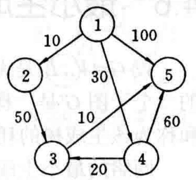
Given a weighted directed graph \(G=(V,E)\), where each edge's weight is a non-negative real number, and a given vertex in \(V\) is designated as the source. Find the shortest path from the source to all other vertices in \(V\). The diagram below illustrates this problem:
2.1.2 Dijkstra's Algorithm
Dijkstra's algorithm is another classic example of the greedy algorithm design strategy. It selects the vertex \(u\) in \(V-S\) with the shortest distance and adds it to \(S\). Then, for each vertex \(v\) in \(V-S\), if there exists an edge from \(u\) to \(v\), it updates the shortest path from the source to \(v\).
We describe Dijkstra's algorithm as follows: given an input weighted directed graph \(G=(V,E), V=\left\{1,2,\cdots,n\right\}\), with vertex \(v\) as the source. A 2D array \(c[i][j]\) is used to represent the weight of edge \((i,j)\). An array \(dist[i]\) is used to store the current shortest path length from the source to vertex \(i\). The basic code is as follows:
1 |
|
The overall time required to complete the algorithm above is \(O(n^2)\).
For the directed graph given in problem description 2.1.1 above, we compute the shortest paths from source vertex 1 to other vertices and trace its iteration process, recorded in the table below:
| Iteration | S | u | dist[2] | dist[3] | dist[4] | dist[5] |
|---|---|---|---|---|---|---|
| Initial | {1} | -- | 10 | maxint | 30 | 100 |
| 1 | {1,2} | 2 | 10 | 60 | 30 | 100 |
| 2 | {1,2,4} | 4 | 10 | 50 | 30 | 90 |
| 3 | {1,2,4,3} | 3 | 10 | 50 | 30 | 60 |
| 4 | {1,2,4,3,5} | 5 | 10 | 50 | 30 | 60 |
For a detailed step-by-step analysis of the algorithm above, refer to this article: Dijkstra's Shortest Path Algorithm - A Visual Introduction
2.2 Minimum Spanning Tree
2.2.1 Problem Description
Let \(G(V,E)\) be an undirected connected weighted graph. The weight of each edge \((v,w)\) in \(E\) is \(c[v][w]\). If a subgraph \(G'\) of \(G\) is a tree containing all vertices of \(G\), then \(G'\) is called a spanning tree of \(G\). Among these, the spanning tree with the minimum total cost (or the minimum total edge weight) is called the Minimum Spanning Tree.
Before solving this problem, we need to understand its properties. Let \(G=(V,E)\) be a connected weighted graph, and let \(U\) be a proper subset of \(V\). If \((u,v)\in E\), \(u\in U\), \(v \in V-U\), and \((u,v)\) has the minimum weight among all such edges crossing the cut, then this edge must belong to a minimum spanning tree of \(G\).
2.2.2 Prim's Algorithm
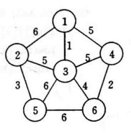
For the aforementioned \(G\), first set \(S=\left\{1\right\}\). As long as \(S\) is a proper subset of \(V\), make the following choice: pick the edge \((i,j)\) with minimum \(c[i][j]\) satisfying \(i \in S\) and \(j \in V-S\), and add vertex \(j\) to \(S\). Repeat until \(S=V\). In simple terms, it involves iteratively adding the "shortest" connecting edge to the spanning tree until all vertices are included, thereby obtaining the minimum spanning tree. Take the following connected weighted graph as an example:
The image below illustrates the process of Prim's algorithm: 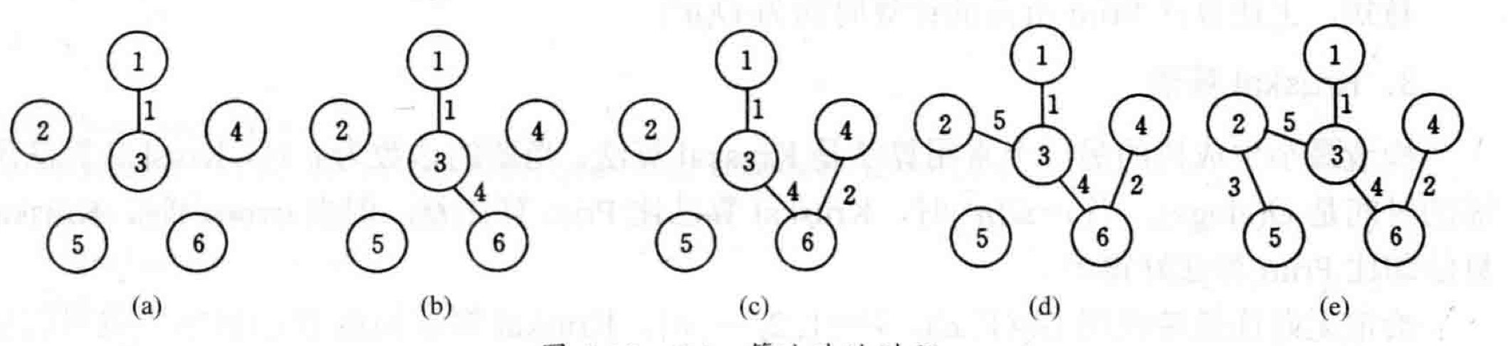
1 |
|
Its time complexity is \(O(n^2)\).
2.2.3 Kruskal's Algorithm
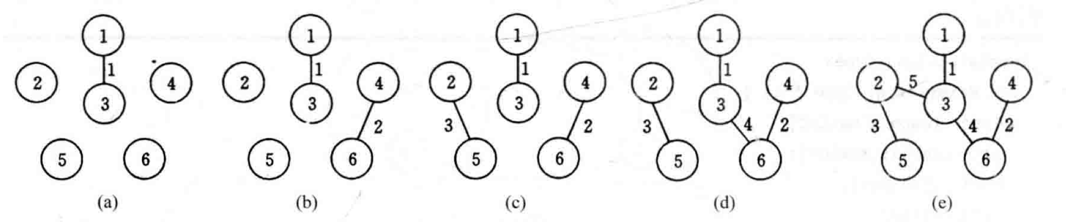
Kruskal's algorithm is another commonly used algorithm for solving the minimum spanning tree problem. If Prim's algorithm starts from adjacent vertices and finds the next vertex by picking the shortest edge, Kruskal's algorithm starts by finding the shortest edges, using edges as the starting point to connect vertices and build the minimum spanning tree.
The basic idea of the algorithm is: initially treat each vertex in the graph as an independent component (or tree). Sort all edges in non-decreasing order of weight, and inspect each edge in sequence to see whether it connects two independent components. If it does, add this edge and the connected vertices to the tree; otherwise, skip it and inspect the next edge. Once all edges have been processed, the minimum spanning tree is obtained.
1 |
|
For a graph with \(e\) edges, constructing the priority queue takes \(O(e)\) time. DeleteMin takes \(O(\log{e})\) time. Implementing UnionFind requires \(O(e \log{e})\) or \(O(e \alpha(e))\) time (where \(\alpha\) is the inverse Ackermann function, often written as \(O(e \log^*{e})\)). Therefore, the overall time complexity of Kruskal's algorithm is \(O(e \log{e})\).
From this, it can be seen that when \(e=\Omega(n^2)\) (dense graph), Kruskal's algorithm performs worse than Prim's algorithm, but when \(e=o(n^2)\) (sparse graph), Kruskal's algorithm performs better than Prim's algorithm.