

Recursion and Divide-and-Conquer Algorithms
1. Basic Algorithmic Concepts
Break down large problems into small ones, simplify complexity, decompose a problem into multiple smaller subproblems of the same type, solve them, and finally merge the results to obtain the solution to the original problem.
For a problem to be solved, if its scale is large or the direct solving process is complicated, we can decompose it into multiple relatively small subproblems to solve. This is the basic idea of recursion. Divide-and-conquer algorithms are an application of recursion. Below, the author will briefly introduce their basic concepts and algorithmic ideas.
1.1 Recursion Algorithm
A so-called recursive algorithm is an algorithm that directly or indirectly calls itself during execution. Below is pseudocode representing a recursive function:
1 |
|
From the pseudocode, we can deduce the basic execution logic of a recursive algorithm: the outer function continually calls deeper into inner layers until it hits the base condition, and then executes and returns layer by layer. The resulting execution process begins at the innermost (or bottom) function call, returning successively to the outer (or upper) layers. The following diagram illustrates this execution process:
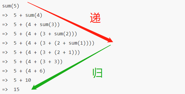
As can be seen, before the outer function executes its functional portion, it first enters inner layers for execution until hitting the base condition (\(sum(1)\) in the figure above), and then executes the actual functional operations from the bottom up.
The advantage of recursive algorithms lies in their concise and easy-to-understand code, enabling bottom-up traversal and execution without using conventional loops. The disadvantage is lower space efficiency, as each recursive call allocates new space in memory; moreover, excessive recursion depth can lead to stack overflow issues.
1.2 Divide and Conquer Algorithm
Note: Divide-and-conquer is an application of recursion, but not all divide-and-conquer algorithms require recursive implementations.The so-called "divide and conquer" means decomposing a large-scale problem that is complex to solve directly into multiple smaller-scale subproblems that can be solved directly using the same simple method. From this, we can see that the mindset of this algorithm is to repeatedly solve smaller subproblems, and then merge the answers of the subproblems into the answer to the large problem. The decomposition structure is shown in the figure below.
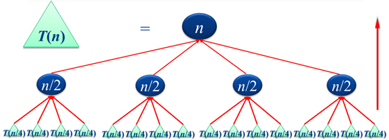
It is easy to see that the order of solving problems can follow a "bottom-up" approach. Therefore, recursive methods can be used to solve them.
Referring to the figure above, let \(n\) be the problem scale, and suppose each step divides into \(k\) subproblems until the subproblem scale is 1. Then the time complexity of merging these problems is \(O(n)\). Thus \(T(n)=kT(n/k)+O(n)\), and the overall time complexity can be reduced to \(O(n\log{n})\).
It should be noted that divide-and-conquer algorithms require the problem to meet the following conditions:
- Each time the problem is divided, the division conditions cannot overlap (they must be mutually exclusive);
- The union of the division conditions must cover all cases of the original problem.
2. Algorithm Applications
Here are several algorithmic applications of recursion and divide-and-conquer strategies.
2.1 Binary Search
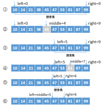
Binary search is a typical application of divide-and-conquer algorithms. In a given sorted array, by comparing the target element with the middle element of the array, the sub-interval containing the target is determined. This operation is then repeated on that sub-interval until the target element is found or the interval becomes empty. Taking searching for the element 47 in a sorted array as an example, the process is shown below:
1 |
|
Complexity Analysis:
As can be seen from the code, each iteration of the while loop halves the size of the search array. In the worst case, the while loop is executed \(O(\log{n})\) times, meaning the worst-case time complexity of the algorithm is \(O(\log n)\).
2.2 Large Integer Multiplication
Multiplication is one of the fundamental operations of computers; however, when handling multiplication of large integers, numerical overflow and excessive computation times often occur. Since direct calculation efficiency falls short of expectations, we can naturally think of decomposing large integers, computing with smaller parts, and merging them to find the answer—that is, using divide and conquer.
Let us use two \(n\)-digit base-\(k\) integers, \(X\) and \(Y\), as an example. We divide each into two segments of \(n/2\) digits, as shown below:

From this, we obtain expressions for \(X\) and \(Y\):
\[ \begin{align*} X=Ak^{n/2}+B\\ Y=Ck^{n/2}+D \end{align*} \]
Then we can obtain \(XY=AC\times{k^n}+(AD+BC)\times{k^{n/2}+BD}\). However, inspecting this formula shows there are still four multiplication operations. To reduce the total number of operations, we simplify further: \(XY=AC\times{k^n}+((A-B)(D-C)+AC+BD)\times{k^{n/2}}+BD\). The actual code implementation only needs to calculate according to this formula:
1 |
|
Complexity Analysis:
Its recurrence relation for time complexity is as follows:
\[ f(x)=\left\{ \begin{aligned} & O(1) && n=1\\ &3T(\frac{n}{2})+O(n) && n>1 \end{aligned} \right. \]
Solving this yields \(O(n^{\log{3}})=O(n^{1.59})\).
2.3 Merge Sort and Quick Sort
2.3.1 Merge Sort
Merge sort is essentially a sorting method that divides first and merges later. Its approach divides the original sequence to be sorted into several sub-sequences of equal size, and then divides each sub-sequence equally again until the sub-sequences are sorted or contain only one element. Then it reverse-merges them into a sorted sequence. The recursive nature of its process is very clear; below is an example of the sorting process:

1 |
|
Time Complexity Analysis:
When sorting \(n\) elements, the Merge and Copy functions can clearly both be completed in \(O(n)\) time. Therefore, in the worst case, the algorithm's running time satisfies: \[ T(n)= \left\{ \begin{aligned} &O(1) &n\leqslant 1\\ &2T(\frac{n}{2})+O(n) &n>1 \end{aligned} \right. \]
From the recurrence equation, we can obtain \(T(n)=O(n\log{n})\).
Algorithm Optimization:
In fact, during merge sort, the sequence set to be sorted is often simply divided into two sub-sequences until only one element remains in each sub-sequence. Therefore, a non-recursive approach can also be used to implement this sort. We divide adjacent elements in the original sequence into pairs, sort within each pair first, and then sort and merge adjacent pairs until all elements are merged. This method is also known as "natural merge sort". Basic reference code is as follows:
1 |
|
Here, the MergePass function is used to merge adjacent sorted arrays.
2.3.2 Quick Sort
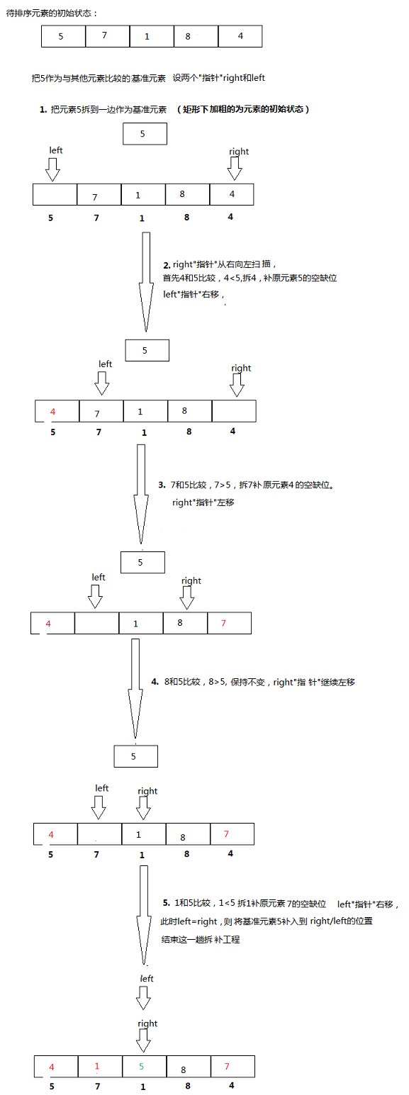
As its name implies, quick sort features favorable time complexity. Its basic idea is to choose a pivot element, place all elements smaller (or larger) than it to its left and all elements larger (or smaller) than it to its right according to the sorting goal. Then the same operation is performed recursively on the left and right sides until all elements are sorted. Taking the following data sorting process as an example:
1 |
|
Time Complexity Analysis:
Clearly, the computing time of the Partition() function is \(O(n)\). For the algorithm as a whole, the worst case occurs when the partition sizes are split into \(n-1\) and \(1\) elements. If this occurs at every step of Partition(), its time complexity satisfies: \[ T(n)= \left\{ \begin{aligned} &O(1) &n\leqslant 1\\ &T(n-1)+O(n) &n>1 \end{aligned} \right. \] This recurrence relation gives: \(T(n)=O(n^2)\).
In the best case, where each pivot happens to be the median, each Partition() satisfies: \[ T(n)= \left\{ \begin{aligned} &O(1) &n\leqslant 1\\ &2T(\frac{n}{2})+O(n) &n>1 \end{aligned} \right. \] This recurrence relation gives: \(T(n)=O(n\log{n})\).
Ultimately, we find that the average time complexity of the quick sort algorithm is \(O(n\log{n})\).
2.4 Linear Time Selection
The problem linear time selection solves is finding the \(k\)-th smallest (or largest) element in a linearly orderable sequence. One approach is to sort all elements using a sorting algorithm and then locate the target element directly in \(O(1)\) time. But clearly, since we only need to find the \(k\)-th smallest (or largest) element, there is no need to sort the entire sequence. Basing our approach on quick sort, but only recursively sorting within the range containing the target element, allows us to avoid wasting time sorting irrelevant parts.
Before introducing this algorithm, we first randomize the partition function from quick sort. This is achieved by randomly choosing a pivot element within the range during each recursive partition, which makes the partition results more balanced and avoids worst-case extremes. Referring to the Partition() function in quick sort above, we can modify it to:
1 |
|
Based on the code above, we can obtain the basic code for linear time selection:
1 |
|
Algorithm Complexity Analysis:
In the worst case, its time complexity is \(O(n^2)\). In the average case, its time complexity is \(O(n)\).
Algorithm Improvement:
In addition to the above method, there is another algorithm that can achieve sorting/selection in \(O(n)\) even in the worst case, generally referred to as Select (Median of Medians). Its steps are:
- Divide the \(n\) elements into \(\lceil n/5 \rceil\) groups, sort each group, and find its median;
- Recursively call the Select function to find the median of the \(\lceil n/5 \rceil\) medians (if \(\lceil n/5 \rceil\) is even, take the larger of the two middle elements), and use this element as the pivot for partitioning.
1 |
|
References
[1] 【Algorithm Learning Notes】Divide and Conquer Algorithm
[2] Recursion and Divide-and-Conquer Strategies (1)
[3] Comparison Sort: Merge Sort