1. Algorithm Complexity Analysis

Algorithm complexity indicates how much computer resources an algorithm consumes. From this, we know that algorithm complexity can be divided into time complexity and space complexity. Given that computer storage space is generally abundant nowadays, we often focus more on the time complexity of an algorithm—that is, the optimization of algorithm efficiency. Therefore, when analyzing algorithm complexity, we mainly discuss the algorithm's time complexity.

1.1 Concretization of the Algorithm Complexity Function

We use \(N\), \(I\), and \(A\) to represent the size of the problem to be solved, the algorithm's input, and the algorithm itself, respectively, and use \(C\) to represent algorithm complexity. Then we can let \(C=F(N,I,A)\). Here, \(F(N,I,A)\) is the complexity function, which is generally determined by the inherent characteristics of the algorithm itself, so we can omit \(A\). For ease of understanding, we replace \(C\) with \(T\) to represent time complexity, yielding the function \(T=T(N,I)\), and analyze this function concretely.

Suppose we have an abstract computer running an algorithm. The smallest operation executed in the algorithm is called an elementary operation. Assume there are \(k\) types of elementary operations, denoted as \(O_1,O_2,\cdots,O_k\), and the execution time for a single run of each elementary operation is \(t_1,t_2,\cdots,t_k\), respectively. Statistically, the number of times the elementary operation \(O_i\) is executed in the algorithm is \(e_i(i=1,2,\cdots,k)\). Note that the execution count \(e_i\) is often related to the problem size and the algorithm input; thus, we have \(e_i=e_i(N,I)\), where \(e_i(N,I)\) is the relation function. From this, we obtain: \[ T(N,I)=\sum_{i=1}^{k}t_ie_i(N,I) \]

where \(t_i(i=1,2,\cdots,k)\) are constants independent of \(N\) and \(I\).

Further concretely, we can consider the best-case, worst-case, and average-case time complexities. In general, the performance of the same algorithm varies according to its input condition \(I\). Therefore, we can easily derive the complexity for the three cases. Let \(\tilde{I}\) be a valid input that allows the algorithm's time complexity to achieve \(T_{min}(N)\), \(I^*\) be a valid input that causes the time complexity to reach \(T_{max}(N)\), and \(P(I)\) be the probability of input \(I\). Then we have:

\[\begin{align*} &T_{min}=\sum_{i=1}^kt_ie_i(N,\tilde{I})=T(N,\tilde{I})\\ &T_{max}=\sum_{i=1}^kt_ie_i(N,I^*)=T(N,I^*)\\ &T_{avg}=\sum_{I\in D_N}P(I)T(N,I)=\sum_{I\in D_N}P(I)\sum_{i=1}^kt_ie_i(N,I) \end{align*}\]

where \(D_N\) is the set of valid inputs of size \(N\).

1.2 Asymptotic Complexity Analysis

When dealing with large-scale algorithms, it is difficult to calculate their exact complexity. Therefore, the concept of asymptotic complexity is introduced to facilitate comparing the efficiency of two algorithms. Taking time complexity \(T(N)\) as an example: for \(T(N)\), if there exists \(\tilde{T}(N)\) such that \(\frac{(T(N)-\tilde{T}(N))}{T(N)}\rightarrow0\) as \(N\rightarrow \infty\), then \(\tilde{T}(N)\) is called the asymptotic complexity of the algorithm as \(N\rightarrow \infty\). Generally, we consider \(\tilde{T}(N)\) to be the simplified expression of \(T(N)\) after removing constant terms and lower-order terms.

For example, given \(T(N)=3N^2+4N\log{N}+7\), then \(3N^2\) is one form of \(\tilde{T}(N)\). We know that when \(N\rightarrow \infty\), we can use \(\tilde{T}(N)\) to approximate \(T(N)\), thereby analyzing and comparing algorithm complexity. Therefore, in the example above, the expression \(3N^2\) can substitute for \(T(N)\) to analyze time complexity. For the asymptotic behavior of a function under different conditions, mathematics provides five notations to define common cases:

• Upper Bound: \(O\) (big O). Let \(f(N)\) and \(g(N)\) be positive functions defined on the set of positive numbers. If there exist positive constants \(C\) and \(N_0\) such that \(f(N)\leq Cg(N)\) when \(N\geq N_0\), then we say that \(g(N)\) is an upper bound of \(f(N)\) as \(N\rightarrow \infty\): \(f(N)=O(g(N))\).

• Lower Bound: \(\Omega\) (big Omega). Let \(f(N)\) and \(g(N)\) be positive functions defined on the set of positive numbers. If there exist positive constants \(C\) and \(N_0\) such that \(f(N)\geq Cg(N)\) when \(N\geq N_0\), then we say that \(g(N)\) is a lower bound of \(f(N)\) as \(N\rightarrow \infty\): \(f(N)=\Omega(g(N))\).

• Same Order / Tight Bound: \(\theta\) (theta). Defined as \(f(N)=\theta(g(N))\) if and only if \(f(N)=O(g(N))\) and \(f(N)=\Omega(g(N))\); we say that \(f(N)\) and \(g(N)\) are of the same order.

• Strict Upper Bound: \(o\) (little o). For any given positive constant \(\varepsilon\), there exists a positive number \(N_0\) such that \(|f(N)|< \varepsilon g(N)\) when \(N\geq N_0\). Then we say that \(g(N)\) is a non-tight upper bound of \(f(N)\) as \(N\rightarrow \infty\): \(f(N)=o(g(N))\).

• Strict Lower Bound: \(\omega\) (little omega). For any given positive constant \(\varepsilon\), there exists a positive number \(N_0\) such that \(|f(N)|> \varepsilon g(N)\) when \(N\geq N_0\). Then we say that \(g(N)\) is a non-tight lower bound of \(f(N)\) as \(N\rightarrow \infty\): \(f(N)=\omega(g(N))\).

2. NP-Completeness Theory

In the content above, we learned how to analyze an algorithm's complexity. Now we need to determine and evaluate the computational complexity of an algorithm. Similar to complexity estimation, it is difficult to determine the actual computing time of an algorithm for a problem, but we can evaluate whether an algorithm is "easy" or "hard" by categorizing algorithm complexity. NP (Non-deterministic Polynomial) completeness theory is a theoretical approach used to classify the "difficulty" of computational problem-solving.

2.1 Class P Problems

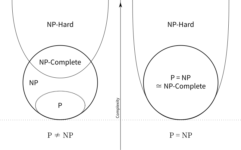
Class P problems (Polynomial Problems) refer to all decision problems that can be solved in polynomial time.

The volume of data involved in computer computing is usually massive, so whether an algorithm's complexity falls within polynomial time often determines whether the algorithm is worth discussing. For class P problems, because their solving time is within polynomial time and the problems addressed are decision problems dealing only with true and false, class P problems can be considered relatively easy to solve. We categorize class P problems as the class of tractable problems under deterministic models.

2.2 Class NP Problems

Class NP problems (Non-deterministic Polynomial Problems) refer to all decision problems whose solutions can be verified in polynomial time.

As mentioned above, class P problems are decision problems that can be solved in polynomial time. In contrast, class NP problems treat the correctness of a problem's solution as a decision problem. The solution to such a problem is non-deterministic, and we cannot compute its solution in polynomial time. However, we can verify whether a given candidate solution is correct in polynomial time. For example: for a given graph, we can verify whether a given path is a Hamiltonian path of the graph in polynomial time.

2.3 Class NP-C Problems

Class NP-Complete problems (Non-deterministic Polynomial Complete Problems) are a special case of class NP problems.

Class NP-C problems are actually more specialized cases within class NP problems. The complexity of these problems is linked to the entire class. If a polynomial-time algorithm exists for any one of these problems, then all NP problems can be solved in polynomial time. In other words, all class NP problems can be reduced to it.

2.4 NP-Hard Problems

NP-hard problems are quite special: they refer to problems to which all class NP problems can be reduced, but which themselves do not necessarily belong to class NP.

2.5 Relationships Among the Four Problem Classes

Regarding class P and class NP problems, their exact relationship has not yet been definitively determined, and the correctness of the statement \(P\neq NP\) is still an open question. Here are Venn diagrams illustrating two possible relationships: