

动态规划(Dynamic Programming)
1.基本算法思想
同样是由大化小解决,但针对的是分解子问题为非独立的情况。
动态规划算法往往用于解决解的最优化问题。其分解的每一级子结构之间往往有重叠,也就是每次产生的子问题并不完全是全新的问题,问题中可能包含有上一级问题的解。为了提高运算效率,在使用该算法时,一般需要使用表格来记录子问题的解,以方便在向上合并时使用它们。通常来说,其可以按照以下步骤进行设计:
- 找出最优解性质,并刻画其结构特征;
- 递归定义最优值;
- 以自底向上的方式计算出最优值;
- 根据计算最优值过程中得到的信息,构造最优解。
动态规划算法的基本要素:
- 最优子结构:如果待解决问题的最优解包含了其子问题的最优解,则称该问题具有最优子结构性质。
- 重叠子问题:在使用动态规划算法时,每次产生的子问题并不完全是全新的问题,问题中可能包含有上一级问题的解。通过上面所提到的表格记录方法解决,一般可以在多项式时间内完成。
- 备忘录方法:这是动态规划算法的一种变形。同样使用表格,备忘录方法使用自顶向下的计算方式,其为每个子问题建立记录项,通过检查记录项确定子问题是否已被计算,如果已经计算则直接使用记录项中的值,否则进行计算并记录。
2.算法应用问题
2.1 矩阵连乘(Matrix Chain Multiplication)
2.1.1 问题描述
给定
矩阵的乘法是满足结合律的,因此可以修改其运算顺序。我们使用加括号的方式来确定矩阵连乘积的运算顺序。
例如,矩阵连乘积
1 | |
2.1.2 算法设计
对于矩阵连乘积
计算最优值:
设计算
其中
对于每一个
1 | |
这里给出《计算机算法设计与分析》一书上的样例方便理解。假设需要计算矩阵连乘积
| 矩阵 | A1 | A2 | A3 | A4 | A5 | A6 |
|---|---|---|---|---|---|---|
| 维数 | 30x35 | 35x15 | 15x5 | 5x10 | 10x20 | 20x25 |
那么其计算顺序以及对应的
例如在计算
计算过程中我们可以知道在
获得最优解:
上面的方法我们仅计算了最少的运算次数,但是还没有得到具体的运算顺序。实际上
例如
1 | |
Trace_back_matrix(1, n, s)
即可获得最优计算顺序。
2.2 最长公共子序列问题(Longest Common Subsequence)
2.2.1 问题描述
给定两个序列
对于这类问题,我们很明显可以知道其具有最优子结构性质。设序列
- 若
,则 ,且 是 和 的最长公共子序列; - 若
,且 ,则 是 和 的最长公子序列; - 若
,且 ,则 是 和 的最长公子序列。
简单理解上述规则,如果在
2.2.2 算法设计
在上面提到的三条规则中,可以知道这个问题带有最优子结构性质和子问题重叠性质。其递归方式如下:
1. 如果
我们建立表
使用表
1 | |
1 | |
该算法的时间复杂度为
实际上,算法中可以省略数据b,因为在
2.3 最大字段和(Maximum Subarray Sum)
2.3.1 问题描述
给定由
在这个问题中,整数序列允许出现负数,因此如果序列所有整数均为负数时,定义其最大子段和为
2.3.2 分治算法解决方法
对于这个问题,我们可以使用分治算法来解决。我们将序列
的最大字段和与 的最大字段和相同; 的最大字段和与 的最大字段和相同; 的最大字段和为 ,且 , 。
对于1、2两种情况,直接进行递归即可。而对于3,我们知道分割点中间两个数一定在最优的序列之中,因此我们可以从分割点向两边扩展,直到序列的两端。这样就可以得到最大字段和。即在
这样的算法复杂度为
1 | |
2.3.3 动态规划解决方法
如果
由此可知,当
该算法时间和空间复杂度都为
1 | |
2.4 0-1背包(0-1 Knapsack)
2.4.1 问题描述
有
2.4.2 算法设计
设
很显然,该问题具有最有子结构性质。我们设0-1背包问题的最优值为
边界条件如下:
我们使用二维表
1 | |
上述代码中,构造出的m[1][c]给出所要求的问题最优值。很显然,算法Knapsack的时间复杂度为
Dynamic Programming
1. Basic Algorithm Idea
It also solves problems by breaking them down from large to small, but it addresses situations where decomposed subproblems are not independent.
Dynamic programming algorithms are often used to solve optimization problems. The substructures at each level of decomposition often overlap, meaning that the subproblems generated each time are not entirely new problems; they may contain solutions to previous level problems. To improve computational efficiency, when using this algorithm, it is generally necessary to use a table to record the solutions to subproblems, making them convenient to use when merging upwards. Generally, it can be designed according to the following steps:
- Identify the properties of an optimal solution and characterize its structural features;
- Recursively define the optimal value;
- Compute the optimal value in a bottom-up manner;
- Construct an optimal solution based on the information obtained during the computation of the optimal value.
Basic elements of dynamic programming algorithms:
- Optimal Substructure: If the optimal solution to the problem to be solved contains the optimal solutions to its subproblems, then the problem is said to possess the optimal substructure property.
- Overlapping Subproblems: When using the dynamic programming algorithm, the subproblems generated each time are not entirely new problems; they may contain solutions to previous level problems. This is typically solved using the table-recording method mentioned above and can generally be completed in polynomial time.
- Memoization: This is a variation of the dynamic programming algorithm. Also using a table, the memoization method uses a top-down computational approach. It creates a record entry for each subproblem, checks the record entry to determine if the subproblem has already been computed, and if so, directly uses the value in the record entry; otherwise, it computes and records it.
2. Algorithm Application Problems
2.1 Matrix Chain Multiplication
2.1.1 Problem Description
Given \(n\) matrices \(\{A_1,A_2,\cdots,A_n\}\), where \(A_i\) and \(A_{i+1}\) are compatible for multiplication (\(i=1,2,\cdots,n-1\)). Find the product \(A_1A_2\cdots A_n\) of these \(n\) matrices.
Matrix multiplication satisfies the associative law, so their order of operations can be changed. We use parenthesizing to determine the order of operations for the matrix chain product.
For example, the matrix chain product \(A_1A_2A_3A_4\) can have the following 5 operation orders: \[ (A_1(A_2(A_3A_4))),(A_1((A_2A_3)A_4)),((A_1A_2)(A_3A_4)),\\ ((A_1(A_2A_3))A_4),(((A_1A_2)A_3)A_4) \] For different operation orders, it is known from the properties of matrix multiplication that the number of operations actually differs. Let \(ra,ca\) and \(rb,cb\) respectively denote matrices \(A,B\). The standard algorithm code for computing their matrix product is as follows:
1 |
|
2.1.2 Algorithm Design
For the matrix chain product \(A_iA_{i+1}\cdots A_j\), let's denote it as \(A[i:j]\). Then for a parenthesizing method \(((A_1\cdots A_k)(A_{k+1}\cdots A_n))\), its number of operations is the product of the operation counts of \(A[1:k]\) and \(A[k+1:n]\) plus their sum.
Calculating the Optimal Value:
Let \(m[i][j]\) be the minimum number of scalar multiplications required to compute \(A[i:j](1\leqslant i\leqslant j \leqslant n)\). Then the optimal solution to the original problem is the value of \(m[1][n]\). For the case where the optimal computation order breaks at \(k(i\leqslant k<j)\), \(m[i][j]\) can be recursively defined as:
\[ m[i][j]= \left\{ \begin{aligned} &0 &i=j \\ &\lim_{i\leqslant k < j} \left \{ m[i][k]+m[k+1][j]+p_{i-1}p_{k}p_{j}\right\} &i<j \end{aligned} \right. \]
Where \(p_i\) represents the number of columns of matrix \(A_i\), and from the properties of matrix product results, it can be known that \(p_{i-1}\) represents the number of rows of matrix \(A_i\).
For each \(k\), there is a corresponding \(m[i][j]\). We create another table \(s[i][j]\) to store the value of \(k\). This way, after obtaining the optimal value \(m[i][j]\), the corresponding optimal solution can be recursively constructed from \(s[i][j]\). We use the recursive formula to compute the \(m\) matrix. Below is the basic code:
1 |
|
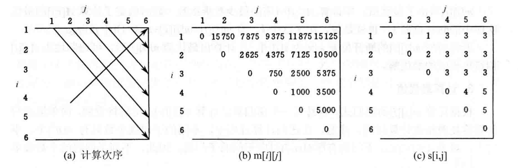
Here's an example from the book "Computer Algorithms: Design and Analysis" for easier understanding. Suppose we need to compute the matrix chain product \(A_1A_2A_3A_4A_5A_6\). Its dimensions are as follows:
| Matrix | A1 | A2 | A3 | A4 | A5 | A6 |
|---|---|---|---|---|---|---|
| Dimensions | 30x35 | 35x15 | 15x5 | 5x10 | 10x20 | 20x25 |
Then its computation order and corresponding \(m\) and \(s\) matrices are as follows:
For example, when calculating \(m[1][3]\), the recursive formula is as follows:
\[\begin{aligned} m[1][3] &= \min \left \{ \begin{aligned} &m[1][1]+m[2][3]+p_0p_1p_3 &=& 0+2625+30\times35\times5=7875 \\ &m[1][2]+m[3][3]+p_0p_2p_3 &=& 15750+0+30\times15\times5=18000 \\ \end{aligned} \right. \\ &=7875 \end{aligned}\]During the calculation, we can see that the smaller value is obtained when \(k=1\), so \(s[1][3]=1\). After the \(m\) matrix is computed, the optimal value \(m[1][n]\) can be obtained.
Obtaining the Optimal Solution:
The method above only calculated the minimum number of operations, but has not yet yielded the specific order of operations. In fact, the data obtained from the \(s\) matrix provides the order information for each calculation.
For example, the information recorded in \(s[1][n]\) indicates that the optimal way to compute \(A[i:n]\) is: \((A[1:s[1][n]])(A[s[1][n]+1:n])\). And the optimal parenthesizing for \(A[1:s[1][n]]\) is: \((A[1:s[1][s[1][n]]])(A[s[1][s[1][n]]+1:s[1][s[1][n]]])\). By iterating this way, the optimal computation order for \(A[1:n]\) is finally determined. Below is the code implementation for this iteration:
1 |
|
Trace_back_matrix(1, n, s), the optimal computation order
can be obtained.
2.2 Longest Common Subsequence
2.2.1 Problem Description
Given two sequences \(X=\{x_1,x_2,\cdots,x_m\}\) and \(Y=\{y_1,y_2,\cdots,y_n\}\), find the longest common subsequence of \(X\) and \(Y\).
For this type of problem, it is clear that it possesses the optimal substructure property. Let \(Z=\left\{z_1,z_2,\cdots,z_k\right\}\) be a longest common subsequence of sequences \(X\) and \(Y\). Then:
- If \(x_m=y_n\), then \(z_k=x_m=y_n\), and \(Z_{k-1}\) is a longest common subsequence of \(X_{m-1}\) and \(Y_{n-1}\);
- If \(x_m\neq y_n\) and \(z_k\neq x_m\), then \(Z\) is a longest common subsequence of \(X_{m-1}\) and \(Y\);
- If \(x_m\neq y_n\) and \(z_k\neq y_n\), then \(Z\) is a longest common subsequence of \(X\) and \(Y_{n-1}\).
To simply understand the above rules, if under the condition \(z_k\neq x_m\) there exists a common subsequence \(W\) with length greater than \(k\), then the length of \(W\) must be greater than \(Z\), and \(W\) would become a common subsequence of \(X\) and \(Y\) with length greater than \(k\). This clearly contradicts \(Z\) being the longest common subsequence of \(X\) and \(Y\). Therefore, \(Z\) is a longest common subsequence of \(X_{m-1}\) and \(Y\). Other cases can be proved by analogy.
2.2.2 Algorithm Design
From the three rules mentioned above, it can be seen that this problem possesses optimal substructure and overlapping subproblems properties. Its recursive approach is as follows: 1. If \(x_m=y_n\), start finding the longest common subsequence of \(X_{m-1}\) and \(Y_{n-1}\), then add \(x_m(x_m=y_n)\) to the end of this subsequence; 2. If \(x_m\neq y_n\), then find a longest common subsequence of \(X_{m-1}\) and \(Y\), and a longest common subsequence of \(X\) and \(Y_{n-1}\) separately. Then compare the lengths of the two longest common subsequences and take the longer one as the longest common subsequence of \(X\) and \(Y\).
We build table \(c\) to record the length of the common subsequence. Suppose we want to determine for sequences \(X_i=\left\{x_1,x_2,\dots,x_i\right\}\) and \(Y_j=\left\{y_1,y_2,\dots,y_j\right\}\). When \(i=0\) or \(j=0\), the empty sequence is their longest common subsequence, so \(c[i][j]=0\). The recursive relation summarized above is as follows:
\[ c[i][j]= \left\{ \begin{aligned} &0 &i>0;j=0 \\ &c[i-1][j-1]+1 &i,j>0;x_i=y_j \\ &\max \left \{ c[i][j-1],c[i-1][j] \right \} &i,j>0;x_i\neq y_j \end{aligned} \right. \]
Use table \(b\) to record which subproblem yielded the corresponding value in \(c\). We obtain the following code based on the recursive relation:
1 |
|
1 |
|
The time complexity of this algorithm is \(O(m+n)\).
In fact, data \(b\) can be omitted in the algorithm, because in table \(c\), element \(c[i][j]\) is often determined by only three elements: \(c[i-1][j-1], c[i-1][j]\) and \(c[i][j-1]\). Therefore, even without table \(b\), we can still know which of the three elements mentioned above determined a certain element.
2.3 Maximum Subarray Sum
2.3.1 Problem Description
Given a sequence \(A=\{a_1,a_2,\cdots,a_n\}\) consisting of \(n\) integers, find the maximum value of a subarray sum of the form \(\sum\limits_{k=i}^{j}a_k\).
In this problem, the sequence of integers is allowed to contain negative numbers. If all integers in the sequence are negative, its maximum subarray sum is defined as \(0\). For example, when \((a_1,a_2,a_3,a_4,a_5,a_6)=(-2,11,-4,13,-5,-2)\), the maximum subarray sum is \(\sum\limits_{k=2}^4a_k=20\).
2.3.2 Divide-and-Conquer Algorithm Solution
For this problem, we can use a divide-and-conquer algorithm to solve it. We divide the sequence \(a(1:n)\) into two equal-length segments and find their maximum subarray sums separately. There are three cases:
- The maximum subarray sum of \(a[1:n]\) is the same as that of \(a[1:\frac{n}{2}]\);
- The maximum subarray sum of \(a[1:n]\) is the same as that of \(a[\frac{n}{2}+1:n]\);
- The maximum subarray sum of \(a[1:n]\) is \(\sum\limits_{k=i}^ja_k\), where \(1\leqslant i\leqslant \frac{n}{2}\) and \(\frac{n}{2}+1\leqslant j\leqslant n\).
For cases 1 and 2, direct recursion is sufficient. For case 3, we know that the two numbers in the middle of the split point must be within the optimal sequence. Therefore, we can extend from the split point outwards to both ends of the sequence. This way, the maximum subarray sum can be obtained. That is, calculate \(s_1=\max\limits_{1\leqslant i\leqslant \frac{n}{2}}\sum\limits_{k=i}^{n/2}a[k]\) in \(a[1:\frac{n}{2}]\), and \(s_2=\max\limits_{\frac{n}{2}+1\leqslant j\leqslant n}\sum\limits_{k=\frac{n}{2}+1}^{j}a[k]\) in \(a[\frac{n}{2}+1:n]\). Then \(s_1+s_2\) is the maximum subarray sum of \(a[1:n]\).
The time complexity of such an algorithm is \(O(n\log n)\). Below is the code implementation:
1 |
|
2.3.3 Dynamic Programming Solution
If \(b[j]=\max\limits_{1\leqslant i \leqslant j} \{ \sum\limits_{k=i}^ja[k]\}(1\leqslant j \leqslant n)\), then the maximum subarray sum sought is \[ \max\limits_{1\leqslant \leqslant i \leqslant j \leqslant n}\sum\limits_{k=i}^j a[k]=\max\limits_{1\leqslant i \leqslant n } \] \[ \max\limits_{1\leqslant i \leqslant j} \sum\limits_{k=i}^ja[k] =\max\limits_{1\leqslant j \leqslant n}b[j] \]
From this, it can be seen that when \(b[j-1]>0\), \(b[j]=b[j-1]+a[j]\); otherwise, \(b[j]=a[j]\). Its recursive formula can be derived as: \[ b[j] = \max\{b[j-1]+a[j],a[j]\} \qquad 1\leqslant j \leqslant n \]
The time and space complexity of this algorithm are both \(O(n)\). The code is as follows:
1 |
|
2.4 0-1 Knapsack
2.4.1 Problem Description
There are \(n\) items and a knapsack with capacity \(c\). Item \(i\) has weight \(w_i\) and value \(v_i\). Determine how to choose items to put into the knapsack to maximize the total value.
2.4.2 Algorithm Design
Let \((y_1,y_2, \cdots ,y_n)\) be an optimal solution to the given 0-1 knapsack problem. Then \((y_2,y_3,\cdots,y_n)\) is an optimal solution to the following corresponding subproblem:
\[ \max{\sum\limits_{i=2}^n v_iy_i} \qquad \left\{ \begin{aligned} &\sum\limits_{i=2}^n w_iy_i \leqslant c-w_1y_1 \\ &x_i \in \{0,1\} \qquad 2\leqslant i \leqslant n \end{aligned} \right. \]
Clearly, this problem has the optimal substructure property. Let \(m(i,j)\) be the optimal value for the 0-1 knapsack problem. Then its recursive formula is: \[ m(i,j)= \left\{ \begin{aligned} &m(i+1,j) &0\leqslant j<w_i \\ &\max \{m(i+1,j),m(i+1,j-w_i)+v_i\} &j\geqslant w_i \end{aligned} \right. \]
The boundary conditions are as follows: \[ m(n,j)= \left\{ \begin{aligned} &0 &0\leqslant j<w_n \\ &v_n &j\geqslant w_n \end{aligned} \right. \]
We use a 2D table \(m\). The basic code is as follows:
1 |
|
In the code above, the constructed \(m[1][c]\) gives the optimal value for the required problem. Clearly, the time complexity of the Knapsack algorithm is \(O(nc)\), and that of Traceback is \(O(n)\).