算法分析笔记:递归与分治策略

2023年08月03日08/03/2023 2.6K 字3K words 大概 10 分钟About 18 min

递归与分治算法

1基本算法思想

由大化小，由繁化简，将一个问题分解为多个规模较小的相同问题进行求解，最后将结果合并，得到原问题的解。

对于一个待解决的问题，如果其规模较大，或者直接的求解过程较为复杂，那么我们就可以将其分解为多个相对较小的子问题进行解决。这就是递归的基本思想。而分治算法则是递归的一种应用。下面笔者将简单介绍它们的基本概念和算法思想。

1.1 递归算法(Recursion Algorithm)

所谓递归算法，就是在过程中直接或间接调用自身的算法。下面给出一段表示递归函数的伪代码：

type recursion(int p_n)                 //p_n为当前递归的参数
{
    if(边界条件) return solve;           //solve为边界条件下的解
    recursion(p_n-1);                   //p_n-1为下一次递归的参数
    ......                              //其他操作
}

通过伪代码我们可以推断出递归算法的基本运行逻辑：外层的函数会不断向内层调用，知道触碰到边界条件，然后逐层执行并返回。最后呈现的运行过程就是由最内层(或者底层)的函数开始执行，逐次返回外层(或上层)。用下图为例简要表示其运行过程：

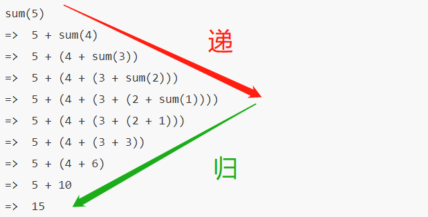
可以看到，在外层函数尚未执行其部分功能部分时，先进入了内层进行执行，直到触碰边界条件(上图中是)，随后由底层向上执行实际功能部分。

递归算法的优势在于其代码表示简洁易懂，无需使用常规循环就可以实现自底向上的遍历运行。其缺点则是较低的空间效率，因为每次递归调用都会在内存中开辟新的空间，而且递归的层数过多时，会导致栈溢出的问题。

1.2 分治算法(Divide and Conquer Algorithm)

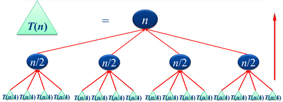
注意：分治算法是递归的应用，但并不是所有分治算法都需要递归实现。

所谓"分治",就是将一个规模较大的，直接求解较为复杂的问题，分解为多个规模较小，且可以使用相同的简单方法直接求解的问题。由此我们可以知道，这种算法的思路就是循环解出小问题，再由小问题的答案合并为大问题的答案。分解结构如下图所示。

很容易得到的是，问题的解决顺序可以服从"自底向上"的原则执行。因此可以使用递归的方法解决。

再根据上图，为问题规模，设每次分解为个子问题，知道子问题规模为1。那么我们合并这些问题的时间复杂度就是。则，整体时间复杂的我们可以化为。

需要注意的是,分治算法需要问题满足以下条件才能使用：

每次分解问题时，分解的条件不能重合(互斥的);
分解条件的并集必须覆盖原问题的所有情况。

2.算法应用问题

这里给出递归与分治策略的几个算法应用

2.1 二分搜索(Binary Search)

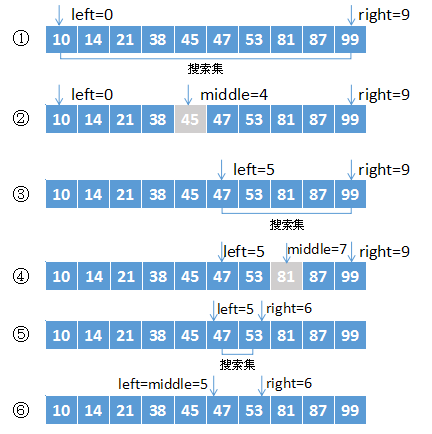
二分搜索是典型的分治算法应用。在已经给出的一个有序序列中，通过比较目标元素与序列中间元素的大小来决定目标所在区间，然后再该区间中重复上述操作，直到找到目标元素或者区间为空。我们以在有序序列中查找47这个元素为例，过程如下图:

二分搜索的基本实现代码:

template<class Type>
int binary_search(Type *arr, const Type &target, int n) //在arr[0,n-1]中查找target

//找到返回下标，否则返回-1
{
    int left = 0, right = n - 1;
    while (left <= right)
    {
        int mid = (left + right) / 2;
        if (arr[mid] == target) 
            return mid;
        else if (arr[mid] > target) 
            right = mid - 1;
        else 
            left = mid + 1;
    }
    return -1;
}

复杂度分析:

由代码可以看出，while循环中每执行一轮，搜索序列的规模就会减半。在最坏的情况下，while循环被执行了此，及算法的时间复杂度最差情况为

2.2 大整数乘法

乘法运算是计算机的基本运算之一，但是在处理较大整数的乘法运算时，往往出现数值溢出，运算时间过长的问题。既然直接计算效率不如预期，我们很自然能够想到将大整数分解，由更小的部分计算合并得出答案，也就是使用分治法。

我们使用两个位进制整数和为例。将它们都分为两端，每段为位，如下图所示

由此我们可以获得与的表达式:

那么就可以得到。但观察该式子，依旧有四次乘法运算。为了简化运算总数，我们再化简，得到:。实际代码实现只要按照改公式计算即可:

//X,Y为两个大整数，n为其位数,k为进制。
//数值类型根据实际情况选择
int big_data_multiple(int X,int Y,int n,int k)
{
    if(n==1) return X*Y;
    int A=X/pow(k,n/2),B=X%pow(k,n/2);
    int C=Y/pow(k,n/2),D=Y%pow(k,n/2);
    int AC=big_data_multiple(A,C,n/2);
    int BD=big_data_multiple(B,D,n/2);
    return AC*pow(k,n)+((A-B)*(D-C)+AC+BD)*pow(,n/2)+BD;
}

复杂度分析:

其时间复杂度方程如下:

得到解为。

2.3 合并排序(Merge Sort)与快速排序(Quick Sort)

2.3.1合并排序

合并排序实际上是一种先分解再合并的排序方法。其方法是将原本的待排序序列等分为几个子序列，然后对每个子序列再进行等分，知道自序列有序或者只有一个元素。然后再将其反合并为有序序列。其过程的递归特征十分明显，以下是一个排序例子的过程:

以下是基本代码:

template <class Type>
void MergeSort(Type *arr, int left, int right) //对arr[left,right]进行排序
{
    if (left <right)
    {
        int mid = (left + right) / 2;
        MergeSort(arr, left, mid);
        MergeSort(arr, mid + 1, right);
        Merge(arr, left, mid, right);
        Copy(arr, left, right);                 //将排序结果复制回原数组
    }
}

时间复杂度分析:

在对n个元素进行排序时，Merge与Copy函数显然都可以在时间内完成，因此在最坏的情况下，算法计算时间满足:

可通过递归方程得到。

算法的优化:

事实上，合并排序过程中往往只是将待排序的序列集合分解为两个子序列，直到子序列剩下一个元素。因此也可以使用非递归方法实现这种排序。我们将原序列中相邻的元素两两分为一组，在每个组中先进行排序，再将相邻的两个组合进行排序和合并，知道所有元素合并完成。这种方法也被称为"自然合并排序"。基本参考代码如下:

template <class Type>
void MergeSort(Type *a, int n)
{
    Type *b = new Type[n];
    int seg = 1;
    while (seg < n)
    {
        MergePass(a, b, seg, n);        //合并至数组b
        seg += seg;
        MergePass(b, a, seg, n);        //合并至数组a
        seg += seg;
    }
}

其中MergePass函数用于合并排序好的相邻数组。

2.3.2快速排序

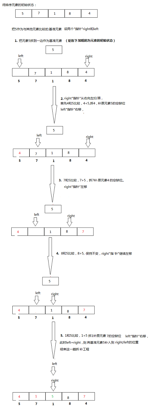
快速排序的性质与其名称一样，拥有较好的时间复杂度。其基本思想是选择一个基准元素，根据排序目标让其左边的元素都小于(或大于)它，右边的元素都大于(或小于)它。然后再对左右两边的元素分别进行同样的操作，直到所有元素都有序。以如下数据排序过程为例:

基本代码如下:

template <class Type>
void QuickSort(Type *a, int p, int r)   //算法主函数
{
    if (p < r)
    {
        int q = Partition(a, p, r);     //获取基准元素的位置
        QuickSort(a, p, q - 1);         //对左边元素进行排序
        QuickSort(a, q + 1, r);         //对右边元素进行排序
    }
}

template <class Type>
int Partiton(Type *a, int p, int r)
{
    int i = p, j = r+1;
    Type x = a[p];                      //基准元素
    while (true)
    {
        while (a[++i] < x && i < r);    //从左向右找到第一个大于x的元素
        while (a[--j] > x);             //从右向左找到第一个小于x的元素
        if (i >= j) break;              //如果两个指针相遇，则退出循环
        swap(a[i], a[j]);               //交换两个元素
    }
    a[p] = a[j];                        //将基准元素放到正确的位置
    a[j] = x;
    return j;                           //返回基准元素的位置
}

时间复杂度分析:

很显然，Partition()函数的计算时间为。对于算法整体而言，其最坏情况出现在区域大小划分为个和个元素的时候。如果Partition()中每一步都是这种情况，那么其时间复杂度满足: 该递归方程得到：。

如果是最好情况，即每次基准数据都恰好为中值，那么每次Partition()就满足: 该递归方程得到：。

最终我们可得到快速排序算法的平均时间复杂度为。

2.4 线性时间选择(Linear Time Selection)

线性时间选择解决的问题是在一个可线性排序的序列中找出第小(或大)的元素。一种解决思路是使用排序算法将所有元素排序，然后直接在时间内找到目标元素。但很显然，因为我们只需要找到第小(或大)的元素，因此没有必要对整个序列进行排序。我们基于快速排序的算法，但只对目标元素所在的范围内进行递归排序，就可以避免浪费时间来对其它不相干部分进行排序。

在介绍该算法之前，我们先对快速排序中的划分函数进行随机化。其体现在每次递归划分时随机选择区域内的基准元素，这样就可以使划分结果更加均匀，避免最坏极端情况出现，参考上面的快速排序中的Partition()函数，我们可以将其改为:

template <class Type>
int RandomizedPartition(Type *a, int p, int r)
{
    int i = p + rand() % (r - p + 1);   //随机选择基准元素
    swap(a[i], a[p]);
    return Partition(a, p, r);
}

基于上述代码，我们可以得到线性时间选择的基本代码:

template <class Type>
int RandomizedSelect(Type *a, int p, int r, int k)
{
    if (p == r) 
        return a[p];
    int i = RandomizedPartition(a, p, r);
    int j = i - p + 1;
    if (k <= j) 
        return RandomizedSelect(a, p, i, k);
    else 
        return RandomizedSelect(a, i + 1, r, k - j);
}

算法复杂度分析:

在最坏情况下，其时间复杂度为。平均情况下，其时间复杂度为。

算法改进:

除了上述方法之外，还有一种最坏情况下也可以用完成排序的算法，一般将其称为Select。其方法步骤为:

将 n 个元素，分成⌈n/5⌉组，对每一组进行排序并取出中位数;
递归调用Select函数，找出⌈n/5⌉个中位数的中位数(若⌈n/5⌉为偶数，则取中间两个数的较大者)，以该元素为基准元素进行划分。

我们设所有元素都不同，找出的基准元素为,那么至少比个元素大，至少比个元素小。此时我们得到对于而言很重要的一个常数分割点,即这个常数。当时，划分的子序列长度至少缩短。因此代码如下:

template <class Type>
Type Select(Type *a,int p, int r, int k)
{
    if(r-p<75)
    {
        对a[p:r]进行排序;
        return a[p+k-1];
    }
    for(int i = 0; i <= (r-p-4)/5; i++)
    {
        将a[p+5*i]至a[p+5*i+4]的第三小元素与a[p+i]交换;
        Type x = Select(a,p,p+(r-p-4)/5,(r-p-4)/10);    //找中位数的中位数
        int i = Partition(a,p,r,x),
            j = i-p+1;
        if(k<=j) 
            return Select(a,p,i,k);
        else
            return Select(a,i+1,r,k-j);
    }
}

参考文献

[1] 【算法学习笔记】之分治算法

[2] 递归与分治策略（1）

[3] Comparison Sort: Merge Sort(合併排序法)

[4] 图解快速排序(By MOBIN)

[5] 线性时间选择算法

Recursion and Divide and Conquer Algorithms

1. Basic Algorithmic Idea

Breaking down a large problem into smaller, simpler, identical problems, solving them, and finally merging the results to obtain the solution to the original problem.

For a problem to be solved, if its scale is large, or the direct solving process is complex, we can decompose it into multiple relatively smaller subproblems. This is the basic idea of recursion. Divide and conquer algorithm, on the other hand, is an application of recursion. Below, the author will briefly introduce their basic concepts and algorithmic ideas.

1.1 Recursion Algorithm

A recursion algorithm is an algorithm that directly or indirectly calls itself during its execution. Below is a pseudocode snippet representing a recursive function:

type recursion(int p_n)                 //p_n is the parameter for the current recursion
{
    if(边界条件) return solve;           //solve is the solution under the boundary condition
    recursion(p_n-1);                   //p_n-1 is the parameter for the next recursion
    ......                              //other operations
}

From the pseudocode, we can deduce the basic execution logic of a recursive algorithm: the outer function continuously calls the inner function until a boundary condition is met, then it executes and returns layer by layer. The final execution process starts from the innermost (or lowest-level) function and returns to the outer (or upper) layers sequentially. The following figure briefly illustrates its execution process:

As can be seen, before the outer function executes its partial functionality, it first enters the inner layer for execution, until the boundary condition is met (which is \(sum(1)\) in the figure above), and then proceeds to execute the actual functional parts from the bottom up.

The advantage of recursive algorithms lies in their concise and easy-to-understand code, enabling bottom-up traversal without using conventional loops. Their disadvantage is lower space efficiency, as each recursive call allocates new space in memory, and too many recursive layers can lead to stack overflow issues.

1.2 Divide and Conquer Algorithm

Note: Divide and conquer algorithms are an application of recursion, but not all divide and conquer algorithms require recursive implementation.

"Divide and conquer" means decomposing a large, complex problem that is difficult to solve directly into multiple smaller problems that can be solved directly using the same simple method. From this, we know that the idea of this algorithm is to repeatedly solve small problems and then merge the solutions of these small problems to get the solution to the large problem. The decomposition structure is shown in the figure below.

It is easy to see that the problem-solving order can follow a "bottom-up" principle. Therefore, it can be solved using recursion.

According to the figure above, \(n\) is the problem size. Assume each decomposition yields \(k\) subproblems, until the subproblem size is 1. Then the time complexity for merging these problems is \(O(n)\). Thus, \(T(n)=kT(n/k)+O(n)\), and the overall time complexity can be simplified to \(O(n\log{n})\).

It should be noted that a divide and conquer algorithm requires the problem to satisfy the following conditions to be applicable:

When decomposing a problem, the decomposition conditions must not overlap (be mutually exclusive);
The union of decomposition conditions must cover all cases of the original problem.

2. Algorithmic Application Problems

Here are several algorithmic applications of recursion and divide and conquer strategies.

2.1 Binary Search

Binary search is a typical application of the divide and conquer algorithm. In a given sorted sequence, it determines the target's interval by comparing the target element with the middle element of the sequence, then repeats the above operation within that interval until the target element is found or the interval is empty. Taking the search for the element 47 in a sorted sequence as an example, the process is shown below:

Basic implementation code for binary search:

template<class Type>
int binary_search(Type *arr, const Type &target, int n) //Search for target in arr[0,n-1]

//Returns index if found, -1 otherwise
{
    int left = 0, right = n - 1;
    while (left <= right)
    {
        int mid = (left + right) / 2;
        if (arr[mid] == target) 
            return mid;
        else if (arr[mid] > target) 
            right = mid - 1;
        else 
            left = mid + 1;
    }
    return -1;
}

Complexity Analysis:

From the code, it can be seen that with each iteration of the while loop, the size of the search sequence is halved. In the worst case, the while loop is executed \(O(\log{n})\) times, meaning the worst-case time complexity of the algorithm is \(O(\log n)\).

2.2 Large Integer Multiplication

Multiplication is one of the basic operations in computers, but when dealing with large integer multiplication, problems such as numerical overflow and excessively long computation times often occur. Since direct calculation is not as efficient as expected, it's natural to think of decomposing large integers, calculating smaller parts, and merging the results to get the answer, which is using the divide and conquer method.

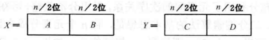
Let's take two \(n\)-digit \(k\)-ary integers \(X\) and \(Y\) as an example. We divide both of them into two parts, each part having \(n/2\) digits, as shown in the figure below:

From this, we can obtain the expressions for \(X\) and \(Y\):

\[ \begin{align*} X=Ak^{n/2}+B\\ Y=Ck^{n/2}+D \end{align*} \]

Then we can get \(XY=AC\times{k^n}+(AD+BC)\times{k^{n/2}+BD}\). However, observing this expression, there are still four multiplication operations. To simplify the total number of operations, we further simplify it to: \(XY=AC\times{k^n}+((A-B)(D-C)+AC+BD)\times{k^{n/2}}+BD\). The actual code implementation just needs to calculate according to this modified formula:

//X,Y are two large integers, n is their number of digits, k is the base.
//Numerical type is chosen based on actual requirements
int big_data_multiple(int X,int Y,int n,int k)
{
    if(n==1) return X*Y;
    int A=X/pow(k,n/2),B=X%pow(k,n/2);
    int C=Y/pow(k,n/2),D=Y%pow(k,n/2);
    int AC=big_data_multiple(A,C,n/2);
    int BD=big_data_multiple(B,D,n/2);
    return AC*pow(k,n)+((A-B)*(D-C)+AC+BD)*pow(,n/2)+BD;
}

Complexity Analysis:

Its time complexity equation is as follows:

\[ f(x)=\left\{ \begin{aligned} & O(1) && n=1\\ &3T(\frac{n}{2})+O(n) && n>1 \end{aligned} \right. \]

The solution obtained is \(O(n^{\log{3}})=O(n^{1.59})\).

2.3 Merge Sort and Quick Sort

2.3.1 Merge Sort

Merge sort is essentially a sorting method that first divides and then merges. Its method is to divide the original sequence to be sorted into several sub-sequences, then further divide each sub-sequence until the sub-sequence is sorted or contains only one element. Then, these are merged back into a sorted sequence. The recursive nature of this process is very obvious. Below is an example of a sorting process:

Here is the basic code:

template <class Type>
void MergeSort(Type *arr, int left, int right) //Sorts arr[left,right]
{
    if (left <right)
    {
        int mid = (left + right) / 2;
        MergeSort(arr, left, mid);
        MergeSort(arr, mid + 1, right);
        Merge(arr, left, mid, right);
        Copy(arr, left, right);                 //Copy sorted result back to original array
    }
}

Time Complexity Analysis:

When sorting \(n\) elements, the Merge and Copy functions can both clearly be completed in \(O(n)\) time. Therefore, in the worst case, the algorithm's computation time satisfies: \[ T(n)= \left\{ \begin{aligned} &O(1) &n\leqslant 1\\ &2T(\frac{n}{2})+O(n) &n>1 \end{aligned} \right. \]

From the recurrence relation, \(T(n)=O(n\log{n})\) can be obtained.

Algorithm Optimization:

In fact, during the merge sort process, the sequence set to be sorted is often only decomposed into two subsequences until each subsequence contains only one element. Therefore, this sorting can also be implemented using a non-recursive method. We group adjacent elements in the original sequence into pairs, sort within each group first, and then sort and merge adjacent groups until all elements are merged. This method is also known as "natural merge sort". The basic reference code is as follows:

template <class Type>
void MergeSort(Type *a, int n)
{
    Type *b = new Type[n];
    int seg = 1;
    while (seg < n)
    {
        MergePass(a, b, seg, n);        //Merge to array b
        seg += seg;
        MergePass(b, a, seg, n);        //Merge to array a
        seg += seg;
    }
}

The MergePass function is used to merge sorted adjacent arrays.

2.3.2 Quick Sort

Quick sort, as its name suggests, has good time complexity. Its basic idea is to choose a pivot element and, according to the sorting objective, ensure that all elements to its left are smaller than (or greater than) it, and all elements to its right are greater than (or smaller than) it. Then, the same operation is performed recursively on the elements to the left and right, until all elements are sorted. Taking the following data sorting process as an example:

The basic code is as follows:

template <class Type>
void QuickSort(Type *a, int p, int r)   //Main algorithm function
{
    if (p < r)
    {
        int q = Partition(a, p, r);     //Get the position of the pivot element
        QuickSort(a, p, q - 1);         //Sort elements on the left
        QuickSort(a, q + 1, r);         //Sort elements on the right
    }
}

template <class Type>
int Partiton(Type *a, int p, int r)
{
    int i = p, j = r+1;
    Type x = a[p];                      //Pivot element
    while (true)
    {
        while (a[++i] < x && i < r);    //Find the first element greater than x from left to right
        while (a[--j] > x);             //Find the first element smaller than x from right to left
        if (i >= j) break;              //If the two pointers meet, exit the loop
        swap(a[i], a[j]);               //Swap the two elements
    }
    a[p] = a[j];                        //Place the pivot element in the correct position
    a[j] = x;
    return j;                           //Return the position of the pivot element
}

Time Complexity Analysis:

Clearly, the computation time of the Partition() function is \(O(n)\). For the algorithm as a whole, its worst case occurs when the region is partitioned into \(n-1\) and \(1\) elements. If every step in Partition() is this situation, then its time complexity satisfies: \[ T(n)= \left\{ \begin{aligned} &O(1) &n\leqslant 1\\ &T(n-1)+O(n) &n>1 \end{aligned} \right. \] This recurrence relation gives: \(T(n)=O(n^2)\).

In the best case, where the pivot data is always exactly the median, then each Partition() satisfies: \[ T(n)= \left\{ \begin{aligned} &O(1) &n\leqslant 1\\ &2T(\frac{n}{2})+O(n) &n>1 \end{aligned} \right. \] This recurrence relation gives: \(T(n)=O(n\log{n})\).

Ultimately, the average time complexity of the quick sort algorithm is \(O(n\log{n})\).

2.4 Linear Time Selection

Linear time selection solves the problem of finding the \(k\)-th smallest (or largest) element in a linearly sortable sequence. One approach is to sort all elements using a sorting algorithm and then find the target element directly in \(O(1)\) time. However, it's clear that since we only need to find the \(k\)-th smallest (or largest) element, there's no need to sort the entire sequence. We can base our solution on the quick sort algorithm, but only recursively sort within the range where the target element is located, thus avoiding wasting time sorting irrelevant parts.

Before introducing this algorithm, let's first randomize the partitioning function in quick sort. This means randomly selecting a pivot element within the region during each recursive partition, which makes the partitioning result more uniform and avoids worst-case extreme scenarios. Referring to the Partition() function in quick sort above, we can modify it as follows:

template <class Type>
int RandomizedPartition(Type *a, int p, int r)
{
    int i = p + rand() % (r - p + 1);   //Randomly select pivot element
    swap(a[i], a[p]);
    return Partition(a, p, r);
}

Based on the above code, we can derive the basic code for linear time selection:

template <class Type>
int RandomizedSelect(Type *a, int p, int r, int k)
{
    if (p == r) 
        return a[p];
    int i = RandomizedPartition(a, p, r);
    int j = i - p + 1;
    if (k <= j) 
        return RandomizedSelect(a, p, i, k);
    else 
        return RandomizedSelect(a, i + 1, r, k - j);
}

Algorithm Complexity Analysis:

In the worst case, its time complexity is \(O(n^2)\). On average, its time complexity is \(O(n)\).

Algorithm Improvement:

In addition to the methods described above, there is also an algorithm that can complete sorting in \(O(n)\) even in the worst case, generally called Select. Its steps are:

Divide \(n\) elements into ⌈n/5⌉ groups, sort each group, and find its median;
Recursively call the Select function to find the median of the ⌈n/5⌉ medians (if ⌈n/5⌉ is even, take the larger of the two middle numbers), and use this element as the pivot for partitioning.

Let's assume all elements are distinct, and the chosen pivot is \(x\). Then \(x\) is greater than at least \(3\times \frac{(n-5)}{10}n\) elements and smaller than at least \(3\times \frac{(n-5)}{10}n\) elements. At this point, we get a crucial constant split point for \(n\), which is \(75\). When \(n\geqslant 75\), the length of the partitioned sub-sequence is reduced by at least \(\frac{1}{4}\). Therefore, the code is as follows:

template <class Type>
Type Select(Type *a,int p, int r, int k)
{
    if(r-p<75)
    {
        对a[p:r]进行排序;
        return a[p+k-1];
    }
    for(int i = 0; i <= (r-p-4)/5; i++)
    {
        将a[p+5*i]至a[p+5*i+4]的第三小元素与a[p+i]交换;
        Type x = Select(a,p,p+(r-p-4)/5,(r-p-4)/10);    //Find the median of medians
        int i = Partition(a,p,r,x),
            j = i-p+1;
        if(k<=j) 
            return Select(a,p,i,k);
        else
            return Select(a,i+1,r,k-j);
    }
}

References

[1] [Algorithm Learning Notes] Divide and Conquer Algorithm

[2] Recursion and Divide and Conquer Strategy (1)

[3] Comparison Sort: Merge Sort(合併排序法)

[4] Illustrated Quick Sort (By MOBIN)

[5] Linear Time Selection Algorithm