算法分析笔记:贪心算法

2023年09月14日09/14/2023 1.6K 字2.3K words 大概 6 分钟About 14 min

贪心算法(Greedy Algorithm)

1.算法基本思想

最优子结构的情况下可用动态规划法，但有时也会有更加简单有效的方法。贪心算法就是在解决子问题时，总是做出当前问题的最好判断。可以说其解决思路是短视和局部的，它并不考虑整体的最优解，只专注于局部问题的解。

上面的描述来看，贪心算法更加直接和高效，但其局限性也很大：很多问题的最优解并不是直接解决其子问题最优解就能得出来的。虽然贪心算法显然不能解决所有问题，但我们依旧可以用它来获得局部的最优解。

1.1 贪心选择性质

上面提到，贪心算法仅在当前问题中做最优解。其选择可以依赖于其曾今的解，但是绝对不会依赖于之后所做的选择。所以该算法通常使用自顶向下的解决顺序。

1.2 贪心算法与动态规划算法的差别

两种算法皆具有最优子结构性质。在笔者的上一篇笔记《算法分析笔记:动态规划》中有提到0-1背包问题。与这个问题类似的一个问题为背包问题。

背包问题

与0-1背包问题类似的，给定种物品，物品的重量是，其价值为，背包容量为。问如何选择物品放入背包，使得背包中物品的总价值最大。但是在背包问题中，可以选择物品的一部分装入背包，而不是全部装入。因此背包问题可以直接根据物品的单位重量价值进行装载。优先装载单位价值高的物品，该物品全部装入背包后如果仍未装满，则选择单位价值次高的物品，直到装满为止。该问题很显然可以使用贪心算法解决，而0-1背包问题不行，因为0-1背包问题不能拆分物品也就意味着其问题的整体最优解不一定对应自顶向下的子问题最优解。算法基础代码如下:

void knapsack(int a, float M, float v[], float w[], float x[])
{
    Sort(n,v,w);
    int i;
    for (i = 1; i <= n; i++)
    {
        x[i] = 0;
    }
    float c = M;
    for (i = 1;i <= n; i++)
    {
        if (w[i] > c)
        {
            break;
        }
        x[i] = 1;
        c -= w[i];
    }
    
    if(i <= n)
    {
        x[i] = c/w[i];
    }
}

上述算法计算时间上界为。

2.算法应用问题

2.1 单源最短路径(Single Source Shortest Path)

2.1.1 问题描述

给定一个带权有向图，每条边的权都是非负实数，给定中的一个顶点称为源。求源到中所有顶点的最短路径。下图是该问题的一个示意图：

2.1.2 Dijkstra算法

Dijkstra算法是贪心算法设计策略的又一个典型例子。在中选择具有最短路线的顶点，并将其加入到中。然后对于每个中的顶点，如果存在一条从到的边，那么就更新从源到的最短路径。

我们这样描述Dijkstra算法：输入带权有向图，源为顶点。使用二维数组表示边的权值。使用数组表示当前从源到顶点的最短路径长度。基本代码如下:

template <class Type>
void Dijkstra(int n, int v, Type dist[], int prev[], Type **c)
{
    bool s[maxint];             // 判断是否已经求得最短路径
    for (int i = 1; i <= n; i++)
    {
        dist[i] = c[v][i];
        s[i] = false;
        if (dist[i] == maxint)
        {
            prev[i] = 0;
        }
        else
        {
            prev[i] = v;
        }
    }
    dist[v] = 0;
    s[v] = true;
    for (int i = 1; i < n; i++)
    {
        Type temp = maxint;
        int u = v;
        for (int j = 1; j <= n; j++)
        {
            if ((!s[j]) && (dist[j] < temp))
            {
                u = j;
                temp = dist[j];
            }
        }
        s[u] = true;
        for (int j = 1; j <= n; j++)
        {
            if ((!s[j]) && (c[u][j] < maxint))
            {
                Type newdist = dist[u] + c[u][j];
                if (newdist < dist[j])
                {
                    dist[j] = newdist;
                    prev[j] = u;
                }
            }
        }
    }
}

以上算法总体需要的时间完成。

对于上面2.2.1问题描述中给出的一个有向图，我们计算从源顶点1到其它顶点的最短路径，推演其迭代过程，使用表格记录:

迭代	S	u	dist[2]	dist[3]	dist[4]	dist[5]
初始	{1}	--	10	maxint	30	100
1	{1,2}	2	10	60	30	100
2	{1,2,4}	4	10	50	30	90
3	{1,2,4,3}	3	10	50	30	60
4	{1,2,4,3,5}	5	10	50	30	60

上述算法具体的过程解析可以参考这篇推文:《图文详解 Dijkstra 最短路径算法》

2.2 最小生成树(Minimum Spanning Tree)

2.2.1 问题描述

设是无向连通带权图。中每条边的权为。如果的一个子图是包含的所有顶点的树，则称为$G的生成树。而其中，其耗费最小的(或者说边最少)生成树即为最小生成树。

解决该问题之前，我们需要了解其的性质。设是连通带权图，是的真子集。如果，且，，且的权值最小，这条边一定存在于的最小生成树中。

2.2.2 Prim算法

对于上面所说的，首先置，只要是的真子集，就做如下选择：选取满足条件的，，且最小的边，并将顶点加入到。直到为止。简单来说，就是将“最短”的连接边加入到生成树中，直到获得完整顶点以得到最小生成树。以下面的连通带权图为例：

下图为Prim算法的图片过程：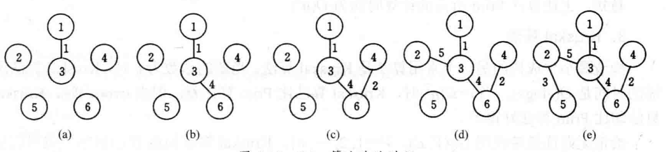

简单来说，该算法将原图打散，从出发点开始，统计所有连接着已经过点和未经过点的边，并找到最短的一条，将其连接的原未经过点加入到已经过点中并循环改过程。下面是基本代码：

template <class Type>
void Prim(int n, Type** c)
{
    Type lowcost[maxint];
    int closest[maxint];
    bool s[maxint];
    s[1] = true;
    for (int i = 2; i <= n; i++)
    {
        lowcost[i] = c[1][i];
        closest[i] = 1;
        s[i] = false;
    }

    for(int i = 1; i < n; i++)
    {
        Type min = inf;
        int j = 1;
        for(int k = 2; k <= n; k++)
        {
            if((lowcost[k] < min) && (!s[k]))
            {
                min = lowcost[k];
                j = k;
            }
        }
    }

    cout << "(" << closest[j] << "," << j << ")" << endl;
    s[j] = ture;
}

其时间复杂度为

。

2.2.3 Kruskal算法

Kruskal算法是解决最小生成树问题的另一种常用算法。如果说Prim算法是以相邻顶点为出发点，通过连接最短边的方式找到下一个点，那么Kruskal算法则是先找最短边，使用以边为出发点找到对应点来构建最小生成树。

算法的基本思想是：先将图中每个顶点看成独立的分支，将所有边按从大到小排列，依次观察该边是否连接了两个独立的分支。如果是，则将该边以及对应顶点加入到树中，否则直接查看下一条。完成所有边的验证后，得到的就是最小生成树。

以下为算法的基本代码：

template <class Type>

class EdgeNode
{
    freind ostream& operator<< (ostream&,EdgeNode<Type>);
    friend bool Kruskal(int, int, EdgeNode<Type>*, EdgeNode<Type>* );
    friend void main(void);
public:
    operator Type() const
    {
        return weight;
    }
private:
    Type weight;
    int u, v;
}

//Kruskal算法
template <class Type>
bool Kruskal(int n, int e, EdgeNode<Type> E[], EdgeNode<Type> t[])
{
    MinHeap<EdgeNode<Type>> H(1); //使用最小堆，用于存放顺序排列的边
    H.Initialize(E, e, e);
    UnionFind UF(n); //这是一个抽象的数据集，可以进行连接或查找操作
    int k = 0;
    while (e && k < n-1)
    {
        EdgeNode<int> x;
        H.DeleteMin(x);
        e--;
        int a = U.Find(x.u);//Find操作，返回集合中对应顶点所在分支的名字
        int b = U.Find(x.v);
        if (a != b)//判断顶点是否在同一分支
        {
            t[k++] = x;
            U.Union(a, b);//Union操作，将两个分支合并
        }
        H.Deactivate(x);
        return (k == n-1);
    }
}

对于一个有条边的图，组成优先队列需要的时间。DeleteMin需要时间。实现UnionFind所需时间为或者。因此Kruskal算法的时间复杂度为。

由此可以看出，当时，Kruskal算法要比Prim算法差，但是当时，Kruskal算法要比Prim算法好。

Greedy Algorithm

1. Basic Idea of the Algorithm

Dynamic programming can be used in cases with optimal substructure, but sometimes there are simpler and more effective methods. A greedy algorithm always makes the best judgment for the current problem when solving subproblems. Its approach can be described as short-sighted and local; it does not consider the overall optimal solution, focusing only on local problem solutions.

From the description above, greedy algorithms are more direct and efficient, but their limitations are also significant: the optimal solution to many problems cannot be derived simply by solving their subproblems optimally. Although greedy algorithms obviously cannot solve all problems, we can still use them to obtain locally optimal solutions.

1.1 Greedy Choice Property

As mentioned above, a greedy algorithm only makes the optimal choice in the current problem. Its choices can depend on previous solutions, but never on future choices. Therefore, this algorithm typically uses a top-down approach.

1.2 Differences Between Greedy Algorithms and Dynamic Programming Algorithms

Both algorithms possess the optimal substructure property. In my previous notes "Algorithm Analysis Notes: Dynamic Programming" I mentioned the 0-1 knapsack problem. A problem similar to this is the knapsack problem.

Knapsack Problem

Similar to the 0-1 knapsack problem, given $n$ items, where item $i$ has weight $w_i$ and value $v_i$, and the knapsack capacity is $c$. The question is how to select items to put into the knapsack to maximize the total value of items in the knapsack. However, in the knapsack problem, a fraction of item $i$ can be put into the knapsack, not just the whole item. Therefore, the knapsack problem can be solved directly by loading items based on their value per unit weight. Items with higher unit value are loaded first. If the knapsack is not full after all of such an item is loaded, the item with the next highest unit value is chosen, and so on, until the knapsack is full. This problem can clearly be solved using a greedy algorithm, while the 0-1 knapsack problem cannot. This is because the inability to split items in the 0-1 knapsack problem means that its overall optimal solution does not necessarily correspond to the optimal solution of its top-down subproblems. The basic algorithm code is as follows:

void knapsack(int a, float M, float v[], float w[], float x[])
{
    Sort(n,v,w);
    int i;
    for (i = 1; i <= n; i++)
    {
        x[i] = 0;
    }
    float c = M;
    for (i = 1;i <= n; i++)
    {
        if (w[i] > c)
        {
            break;
        }
        x[i] = 1;
        c -= w[i];
    }
    
    if(i <= n)
    {
        x[i] = c/w[i];
    }
}

The time complexity of the above algorithm is $O(n \log{n})$.

2. Algorithm Application Problems

2.1 Single Source Shortest Path

2.1.1 Problem Description

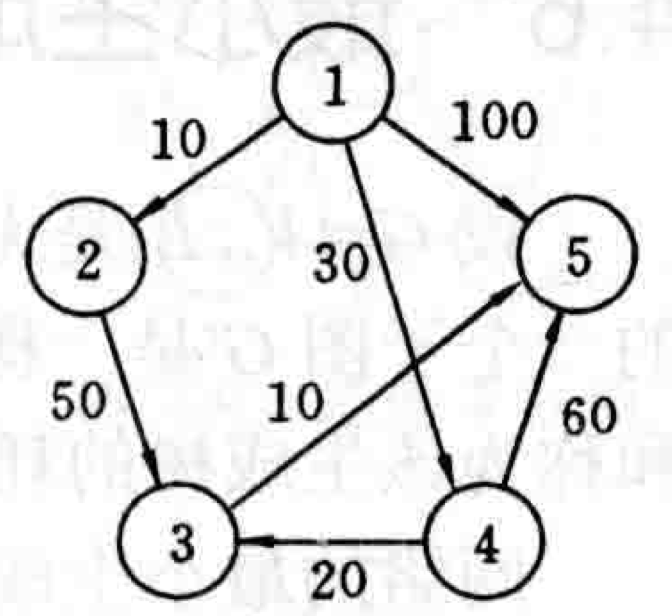
Given a weighted directed graph $G=(V,E)$, where the weight of each edge is a non-negative real number, and a vertex in $V$ is given as the source. Find the shortest paths from the source to all other vertices in $V$. The following image is a schematic diagram of this problem:

2.1.2 Dijkstra's Algorithm

Dijkstra's algorithm is another classic example of a greedy algorithm design strategy. It selects the vertex $u$ with the shortest path in $V-S$ and adds it to $S$. Then, for each vertex $v$ in $V-S$, if there is an edge from $u$ to $v$, it updates the shortest path from the source to $v$.

We describe Dijkstra's algorithm as follows: Given a weighted directed graph $G=(V,E)$, where $V=\left\{1,2,\cdots,n\right\}$ and the source is vertex $v$. A 2D array $c[i][j]$ represents the weight of edge $(i,j)$. An array $dist[i]$ represents the current shortest path length from the source to vertex $i$. The basic code is as follows:

template <class Type>
void Dijkstra(int n, int v, Type dist[], int prev[], Type **c)
{
    bool s[maxint];             // 判断是否已经求得最短路径
    for (int i = 1; i <= n; i++)
    {
        dist[i] = c[v][i];
        s[i] = false;
        if (dist[i] == maxint)
        {
            prev[i] = 0;
        }
        else
        {
            prev[i] = v;
        }
    }
    dist[v] = 0;
    s[v] = true;
    for (int i = 1; i < n; i++)
    {
        Type temp = maxint;
        int u = v;
        for (int j = 1; j <= n; j++)
        {
            if ((!s[j]) && (dist[j] < temp))
            {
                u = j;
                temp = dist[j];
            }
        }
        s[u] = true;
        for (int j = 1; j <= n; j++)
        {
            if ((!s[j]) && (c[u][j] < maxint))
            {
                Type newdist = dist[u] + c[u][j];
                if (newdist < dist[j])
                {
                    dist[j] = newdist;
                    prev[j] = u;
                }
            }
        }
    }
}

The above algorithm generally takes $O(n^2)$ time to complete.

For the directed graph given in the problem description 2.2.1 above, we compute the shortest paths from source vertex 1 to other vertices, trace its iterative process, and record it in a table:

Iteration	S	u	dist[2]	dist[3]	dist[4]	dist[5]
Initial	{1}	--	10	maxint	30	100
1	{1,2}	2	10	60	30	100
2	{1,2,4}	4	10	50	30	90
3	{1,2,4,3}	3	10	50	30	60
4	{1,2,4,3,5}	5	10	50	30	60

For a detailed explanation of the above algorithm, refer to this article: "Dijkstra's Shortest Path Algorithm: A Visual Introduction"

2.2 Minimum Spanning Tree

2.2.1 Problem Description

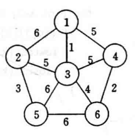
Let $G(V,E)$ be an undirected, connected, weighted graph. The weight of each edge $(v,w)$ in $E$ is $c[v][w]$. If a subgraph $G'$ of $G$ is a tree that includes all vertices of $G$, then $G'$ is called a spanning tree of $G$. Among these, the spanning tree with the minimum cost (or fewest edges) is called the minimum spanning tree.

Before solving this problem, we need to understand its properties. Let $G=(V,E)$ be a connected, weighted graph, and $U$ be a proper subset of $V$. If $(u,v)\in E$, $u\in U$, and $v \in V-U$, and the weight of $(u,v)$ is minimal, then this edge must exist in the minimum spanning tree of $G$.

2.2.2 Prim's Algorithm

For the graph $G$ mentioned above, first set $S=\left\{1\right\}$. As long as $S$ is a proper subset of $V$, make the following choice: select an edge $(i,j)$ such that $i \in S$, $j \in V-S$, and $c[i][j]$ is minimal, then add vertex $j$ to $S$. Repeat until $S=V$. Simply put, it means adding the "shortest" connecting edge to the spanning tree until all vertices are included to form the minimum spanning tree. Consider the following connected weighted graph as an example:

The image below illustrates the process of Prim's algorithm:

Simply put, this algorithm breaks down the original graph, starts from a designated point, counts all edges connecting visited points and unvisited points, finds the shortest one, adds the originally unvisited point connected by this shortest edge to the set of visited points, and repeats this process. Here is the basic code:

template <class Type>
void Prim(int n, Type** c)
{
    Type lowcost[maxint];
    int closest[maxint];
    bool s[maxint];
    s[1] = true;
    for (int i = 2; i <= n; i++)
    {
        lowcost[i] = c[1][i];
        closest[i] = 1;
        s[i] = false;
    }

    for(int i = 1; i < n; i++)
    {
        Type min = inf;
        int j = 1;
        for(int k = 2; k <= n; k++)
        {
            if((lowcost[k] < min) && (!s[k]))
            {
                min = lowcost[k];
                j = k;
            }
        }
    }

    cout << "(" << closest[j] << "," << j << ")" << endl;
    s[j] = ture;
}

Its time complexity is $O(n^2)$.

2.2.3 Kruskal's Algorithm

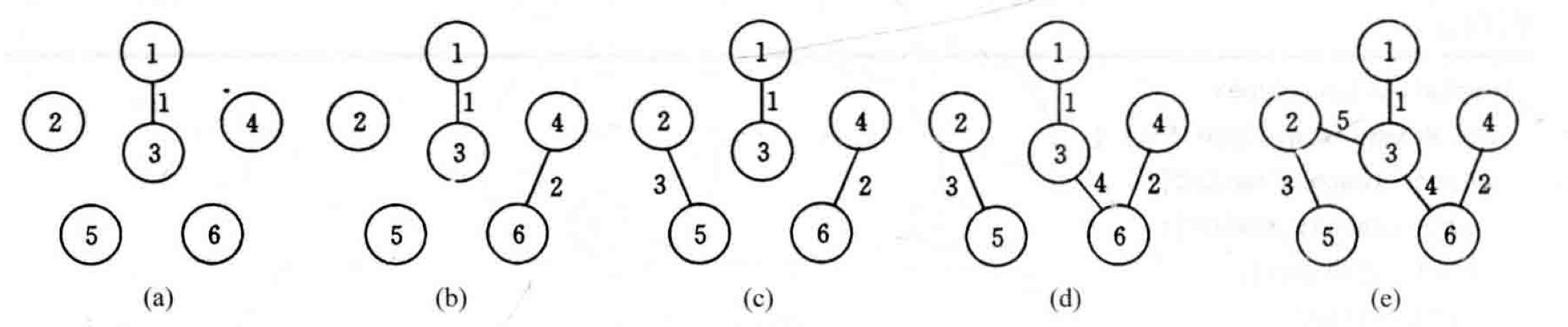
Kruskal's algorithm is another commonly used algorithm for solving the minimum spanning tree problem. While Prim's algorithm starts from an adjacent vertex and finds the next point by connecting the shortest edge, Kruskal's algorithm first finds the shortest edge and uses the edge as a starting point to find the corresponding points to build the minimum spanning tree.

The basic idea of the algorithm is: first, treat each vertex in the graph as an independent component. Arrange all edges in ascending order (smallest to largest). Then, one by one, check if each edge connects two independent components. If it does, add that edge and its corresponding vertices to the tree; otherwise, proceed to the next edge. After verifying all edges, the result is the minimum spanning tree.

The basic code for the algorithm is as follows:

template <class Type>

class EdgeNode
{
    freind ostream& operator<< (ostream&,EdgeNode<Type>);
    friend bool Kruskal(int, int, EdgeNode<Type>*, EdgeNode<Type>* );
    friend void main(void);
public:
    operator Type() const
    {
        return weight;
    }
private:
    Type weight;
    int u, v;
}

//Kruskal算法
template <class Type>
bool Kruskal(int n, int e, EdgeNode<Type> E[], EdgeNode<Type> t[])
{
    MinHeap<EdgeNode<Type>> H(1); //使用最小堆，用于存放顺序排列的边
    H.Initialize(E, e, e);
    UnionFind UF(n); //这是一个抽象的数据集，可以进行连接或查找操作
    int k = 0;
    while (e && k < n-1)
    {
        EdgeNode<int> x;
        H.DeleteMin(x);
        e--;
        int a = U.Find(x.u);//Find操作，返回集合中对应顶点所在分支的名字
        int b = U.Find(x.v);
        if (a != b)//判断顶点是否在同一分支
        {
            t[k++] = x;
            U.Union(a, b);//Union操作，将两个分支合并
        }
        H.Deactivate(x);
        return (k == n-1);
    }
}

For a graph with $e$ edges, forming the priority queue takes $O(e)$ time. DeleteMin takes $O(\log e)$ time. The time required to implement UnionFind is $O(e \log e)$ or $O(e \log^* e)$. Therefore, Kruskal's algorithm has a time complexity of $O(e \log e)$.

From this, it can be seen that when $e=\Omega(n^2)$, Kruskal's algorithm performs worse than Prim's algorithm, but when $e=o(n^2)$, Kruskal's algorithm performs better than Prim's algorithm.