算法分析笔记:复杂度分析与NP完全性理论

2023年07月28日07/28/2023 1.6K 字1.5K words 大概 6 分钟About 9 min

1. 算法复杂度分析

算法复杂度说明了该算法占用计算机资源的多少。由此我们能知道，算法复杂度有时间和空间之分。而在如今计算机存储空间普遍较大的情况下，我们往往更加注重算法时间复杂度，即算法效率的优化。因此在算法复杂度分析时，我们主要讨论算法的时间复杂度。

1.1 算法复杂度函数的具体化

我们使用 $、、$ 来分别表示一个算法需要解的问题的规模、算法的输入和算法本身，使用来表示算法复杂性。那么我们可以令。其中的就是复杂度函数，其一般由算法本身特性得出，因此我们可以将省略。为了方便理解，我们将用来替换，表示时间复杂度，得到函数，并将该函数具体化分析。

我们假设有一台抽象的计算机，并在上面运行一个算法。算法中执行的最小运算我们称为元运算。我们设有种元运算，分别记为，每一种元运算单词执行时间分别为。经过统计，算法中元运算使用的次数为。需要注意的是，使用次数往往和问题的规模以及算法输入有关，因此我们可以得出，其中即为关系函数。由此可得:

其中是与和无关的常数。

进一步具体化的，我们可以考虑最好，最坏情况和平均的时间复杂度。一般情况下，同种算法的复杂度好坏是根据其输入条件变化的。因此我们很容易得出其三种状况的复杂度情况。我们设是能使算法时间复杂度达到的合法输入，是能使时间复杂度达到的合法输入，是输入为的概率。那么我们能得到:

其中,是规模为的合法输入集合。

1.2 渐进复杂度的分析

在面对一些较大规模的算法时，我们很难去计算其具体的复杂度。因此需要引入渐进复杂度的概念来方便我们比较两种算法的效率。同样以时间复杂度为例。对于，如果存在，当时，可以使得，就称为该算法当时的渐进复杂度。一般我们认为就是式子中去掉常数项和低次项后的简单结果。

例如，有，那么就是的一种情况。我们可以知道，当时，我们可以使用来近似，由此来分析对比算法复杂度。所以在上面的例子中，这个式子可以代替来分析时间复杂度。针对一个函数的在不同情况渐进意义，在数学上会给出五种符号来定义常见的情况:

上界: (big O)。令和是定义在正数集上的正函数，如果存在正数和，使得当时有，那么我们就说在时，是的一个上界:。
下界: (big Omega)。令和是定义在正数集上的正函数，如果存在正数和，使得当时，有，那么我们就说在时，是的一个下界:。
同阶: (theta)。定义当且仅当且时，称和是同阶的。
严格上界: (little o)。对于任意给定的正数,都存在正数，使得当时，有，那么我们就说在时，是的一个非紧上界:。
严格下界: (little omega)。对于任意给定的正数,都存在正数，使得当时，有，那么我们就说在时，是的一个非紧下界:。

2. NP完全性理论

在上面的内容中，我们了解了如何去分析一个算法的复杂度，此时我们就要来确认和评价一个算法的计算复杂性。与复杂度估算类似的，我们很难去判断一个问题中算法的实际计算时间，但可以通过对算法复杂度的分类来评价一个算法是“简单”还是“困难”。NP(Non-deterministic Polynomial)完全性理论就是用于区分计算求解“难易度”的理论方法。

2.1 P类问题

P类问题(Polynomial Problem)是指所有可以在多项式时间内求解的判定问题。

计算机计算所涉及的数据量通常是十分巨大的，因此算法复杂度是否是在多项式时间以内往往决定了该种算法是否具备讨论的价值。对于P类问题而言，因为其求解时间在多项式时间内，且解决的问题是只针对true和flase的判断问题，因此可以认为P类问题是比较容易求解的问题。我们将P类问题归类于确定性模型下的易解决问题类。

2.2 NP类问题

NP类问题(Non-deterministic Polynomial Problem)是指所有可以在多项式时间内验证的判定问题。

上面提到，P类问题是可以在多项式时间内求解的判断问题。而NP类问题则是将问题的解的正确性作为一个判断问题。这个问题的解是非确定性的，我们无法在多项式时间内求出它的解。但是我们可以在多项式时间内验证一个已经给出的解是否为正解。例如：对于一个给定的图，我们可以在多项式时间内验证一个给定的路径是否为该图的哈密顿路径。

2.3 NP-C类问题

NP完全类问题(Non-deterministic Polynomial Complete Problem)是NP类问题的特殊情况。

NP-C类问题实际上是NP类问题中更加特殊的情况。这些问题的复杂度与整个类都有关联。如果这些问题中任何一个存在着可以多项式时间内的算法，那么所有的NP问题都可以在多项式时间内求解出来。或者说所有的NP类问题都可以约化(reduce to)为它。

2.4 NP-hard问题

NP-hard问题较为特殊，它指的是所有NP类问题都可以约化为它，但其本身却不属于NP类的问题。

2.5 上四类问题的关系

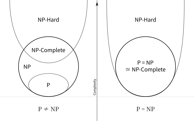
对于P类和NP类问题，目前还没有找到其具体准确的关系，针对这个式子的正确性的问题目前仍然在争论。这里先给出两种可能的关系维恩图:

1. Algorithm Complexity Analysis

Algorithm complexity describes how much computer resources an algorithm consumes. From this, we know that algorithm complexity is divided into time and space. In the current situation where computer storage space is generally large, we often pay more attention to algorithm time complexity, i.e., the optimization of algorithm efficiency. Therefore, in algorithm complexity analysis, we mainly discuss the time complexity of algorithms.

1.1 Specification of the Algorithm Complexity Function

We use $N, I, A$ to represent the size of the problem to be solved by an algorithm, the input of the algorithm, and the algorithm itself, respectively. We use $C$ to represent the algorithm complexity. Then we can let $C=F(N,I,A)$. The $F(N,I,A)$ is the complexity function, which is generally derived from the characteristics of the algorithm itself, so we can omit $A$. For ease of understanding, we replace $C$ with $T$ to represent time complexity, obtaining the function $T=T(N,I)$, and we will analyze this function specifically.

Let's assume there is an abstract computer on which an algorithm runs. The smallest operation executed in the algorithm is called an elementary operation. Suppose there are $k$ types of elementary operations, denoted as $O_1,O_2,\cdots,O_k$, and the execution time of each elementary operation is $t_1,t_2,\cdots,t_k$ respectively. After statistics, the number of times elementary operation $O_i$ is used in the algorithm is $e_i(i=1,2,\cdots,k)$. It is important to note that the number of uses $e_i$ is often related to the problem size and algorithm input, so we can conclude $e_i=e_i(N,I)$, where $e_i(N,I)$ is the relation function. Thus we can get: \[ T(N,I)=\sum_{i=1}^{k}t_ie_i(N,I) \]

Where $t_i(i=1,2,\cdots,k)$ are constants independent of $N$ and $I$.

Further specifying, we can consider the best, worst, and average-case time complexity. Generally, the quality of the complexity of the same algorithm varies according to its input conditions $I$. Therefore, it is easy for us to derive the complexity situations for its three scenarios. Let $\tilde{I}$ be a legal input that minimizes the algorithm's time complexity to $T_{min}(N)$, $I^*$ be a legal input that maximizes the time complexity to $T_{max}(N)$, and $P(I)$ be the probability of input $I$. Then we can get:

\[\begin{align*} &T_{min}=\sum_{i=1}^kt_ie_i(N,\tilde{I})=T(N,\tilde{I})\\ &T_{max}=\sum_{i=1}^kt_ie_i(N,I^*)=T(N,I^*)\\ &T_{avg}=\sum_{I\in D_N}P(I)T(N,I)=\sum_{I\in D_N}P(I)\sum_{i=1}^kt_ie_i(N,I) \end{align*}\]

Where $D_N$ is the set of legal inputs of size $N$.

1.2 Analysis of Asymptotic Complexity

When dealing with algorithms of a larger scale, it is difficult for us to calculate their specific complexity. Therefore, the concept of asymptotic complexity needs to be introduced to facilitate our comparison of the efficiency of two algorithms. Taking time complexity $T(N)$ as an example again. For $T(N)$, if there exists $\tilde{T}(N)$ such that when $N\rightarrow \infty$, $\frac{(T(N)-\tilde{T}(N))}{T(N)}\rightarrow0$, then $\tilde{T}(N)$ is called the asymptotic complexity of this algorithm when $N\rightarrow \infty$. Generally, we consider $\tilde{T}(N)$ to be the simplified result of $T(N)$ after removing constant terms and lower-order terms.

For example, if $T(N)=3N^2+4N\log{N}+7$, then $3N^2$ is a case of $\tilde{T}(N)$. We can know that when $N\rightarrow \infty$, we can use $\tilde{T}(N)$ to approximate $T(N)$, and thus analyze and compare algorithm complexity. So in the above example, the expression $3N^2$ can replace $T(N)$ to analyze time complexity. For the asymptotic meaning of a function in different situations, mathematics provides five symbols to define common cases:

Upper Bound: $O$(big O). Let $f(N)$ and $g(N)$ be positive functions defined on the set of positive numbers. If there exist positive numbers $C$ and $N_0$ such that for $N\geq N_0$, $f(N)\leq Cg(N)$, then we say that $g(N)$ is an upper bound for $f(N)$ as $N\rightarrow \infty$: $f(N)=O(g(N))$.
Lower Bound: $\Omega$(big Omega). Let $f(N)$ and $g(N)$ be positive functions defined on the set of positive numbers. If there exist positive numbers $C$ and $N_0$ such that for $N\geq N_0$, $f(N)\geq Cg(N)$, then we say that $g(N)$ is a lower bound for $f(N)$ as $N\rightarrow \infty$: $f(N)=\Omega(g(N))$.
Tight Bound: $\theta$(theta). $f(N)=\theta(g,(N))$ if and only if $f(N)=O(g(N))$ and $f(N)=\Omega(g(N))$. In this case, $f(N)$ and $g(N)$ are said to be of the same order.
Strict Upper Bound: $o$(little o). For any given positive number $\varepsilon$, there exists a positive number $N_0$ such that for $N\geq N_0$, $|f(N)|< \varepsilon g(N)$. Then we say that $g(N)$ is a non-tight upper bound for $f(N)$ as $N\rightarrow \infty$: $f(N)=o(g(N))$.
Strict Lower Bound: $\omega$(little omega). For any given positive number $\varepsilon$, there exists a positive number $N_0$ such that for $N\geq N_0$, $|f(N)|> \varepsilon g(N)$. Then we say that $g(N)$ is a non-tight lower bound for $f(N)$ as $N\rightarrow \infty$: $f(N)=\omega(g(N))$.

2. NP-Completeness Theory

In the above content, we understood how to analyze the complexity of an algorithm. Now we need to confirm and evaluate the computational complexity of an algorithm. Similar to complexity estimation, it is difficult for us to judge the actual computation time of an algorithm for a problem, but we can evaluate whether an algorithm is "simple" or "difficult" by classifying its complexity. NP (Non-deterministic Polynomial) completeness theory is a theoretical method used to distinguish the "difficulty" of computational problem-solving.

2.1 P-class Problems

P-class problems (Polynomial Problem) refer to all decision problems that can be solved in polynomial time.

The amount of data involved in computer calculations is usually enormous, so whether the algorithm complexity is within polynomial time often determines whether the algorithm is worth discussing. For P-class problems, because their solution time is within polynomial time, and the problems solved are only decision problems (true or false), P-class problems can be considered relatively easy to solve. We classify P-class problems as easily solvable problems under a deterministic model.

2.2 NP-class Problems

NP-class problems (Non-deterministic Polynomial Problem) refer to all decision problems whose solutions can be verified in polynomial time.

As mentioned above, P-class problems are decision problems that can be solved in polynomial time. NP-class problems, on the other hand, treat the correctness of a problem's solution as a decision problem. The solution to this problem is non-deterministic; we cannot find its solution in polynomial time. However, we can verify whether a given solution is correct in polynomial time. For example: for a given graph, we can verify whether a given path is a Hamiltonian path for that graph in polynomial time.

2.3 NP-Complete Problems

NP-Complete problems (Non-deterministic Polynomial Complete Problem) are a special case of NP-class problems.

NP-Complete problems are actually a more special case of NP-class problems. The complexity of these problems is related to the entire class. If any of these problems has an algorithm that runs in polynomial time, then all NP problems can be solved in polynomial time. In other words, all NP-class problems can be reduced to them.

2.4 NP-hard Problems

NP-hard problems are special in that all NP-class problems can be reduced to them, but they themselves do not belong to the NP-class.

2.5 Relationship between the above four types of problems

For P-class and NP-class problems, their specific and accurate relationship has not yet been found, and the correctness of the equation $P\neq NP$ is still debated. Here are two possible Venn diagrams of their relationships: