
Involution is a neural network operator proposed by Li et al. in 2021. It is designed with characteristics opposite to standard convolution, and is often referred to as an inverse-style convolutional operator.
This post records my study and implementation notes from undergraduate thesis work, including core ideas, structural modifications, and early parallelization attempts for acceleration.
Foreword
The author of the technical paper discussed in this article currently faces some controversy regarding academic misconduct; however, this specific paper itself has not been confirmed to involve any problematic content. This post is solely for study and recording purposes. If this paper or its techniques are later proven to involve academic integrity issues, this post will be permanently archived or removed.
Preliminary Introduction
In machine learning, convolution is one of the most classic operations, especially in the field of computer vision (CV). We can briefly review the 2D convolution operation, which extracts features from 2D data by sliding a kernel across it. Before diving into Involution, we need to understand several characteristics of traditional convolution. The convolution operation slides shared convolution kernels across spatial locations, a design featuring two core properties: spatial-agnostic and channel-specific.
Spatial-agnostic means the same convolution kernel is applied to all spatial positions across the feature map; regardless of the location, the weights used remain identical. While this design is parameter-efficient, it limits the model's ability to adaptively model different spatial locations. Channel-specific means convolution learns independent kernels for each output channel, introducing redundancy across convolution kernels.
The Involution operator is designed based on the inverse characteristics of convolution, possessing spatial-specific and channel-agnostic properties. This means Involution generates dedicated kernels for each spatial location that are shared across the channel dimension, offering the following advantages:
- Enhanced adaptability: Each pixel location has its own processing kernel, allowing it to better capture local context information;
- Improved parameter efficiency: The channel sharing mechanism drastically reduces the parameter count, especially in deep networks with large channel numbers;
- Long-range dependency modeling: By expanding the kernel size, Involution can efficiently model long-range spatial relationships while reducing the loss of close-range information, balancing feature extraction capabilities across both near and distant scales.
Simply put, this operator generates adaptive kernels at each position, while channels are grouped to determine which channels share a common kernel. In this way, distinct kernels are utilized for each element while avoiding redundancy generated across different channels. Next, the author will briefly explain its principles.
Overview of Principles
Taking 2D data as an example, for an input feature map \(\mathbf{X} \in \mathbb{R}^{H \times W \times C}\), the output of Involution at position \((i, j)\) can be represented as:
\[ Y_{i,j}= \sum_{(u,v)\in\mathcal{N}(i,j)} \mathcal{H}_{i,j,u,v} \cdot \mathbf{X}_{u,v} \]
where \(\mathcal{N}(i,j)\) is the
neighborhood centered at \((i,j)\), and
\(\mathcal{H}_{i,j} \in \mathbb{R}^{K \times K
\times C}\) is the involution kernel at that position. Its kernel
mapping function is defined as: \[
\phi = \mathbb{R}^C \mapsto \mathbb{R}^{K\times K\times G}
\] This expression implies that the kernel mapping takes channels
as the input dimension and maps them to a three-dimensional form of
kernel size multiplied by groups. It can be understood as performing the
kernel mapping operation based on the channel vector corresponding to
the element location. The specific expression is given below: \[
\mathcal{H}_{i,j} =
\phi(\mathbf{X}_{i,j})=W_1\sigma(W_0\mathbf{X}_{i,j})
\] where \(W_0\) and \(W_1\) are two linear transformations, and
\(\sigma\) represents an activation
function. After obtaining the kernel parameters through the above
mapping, they are applied to the original data to complete the kernel
operation. Below is the schematic diagram used in the original paper:
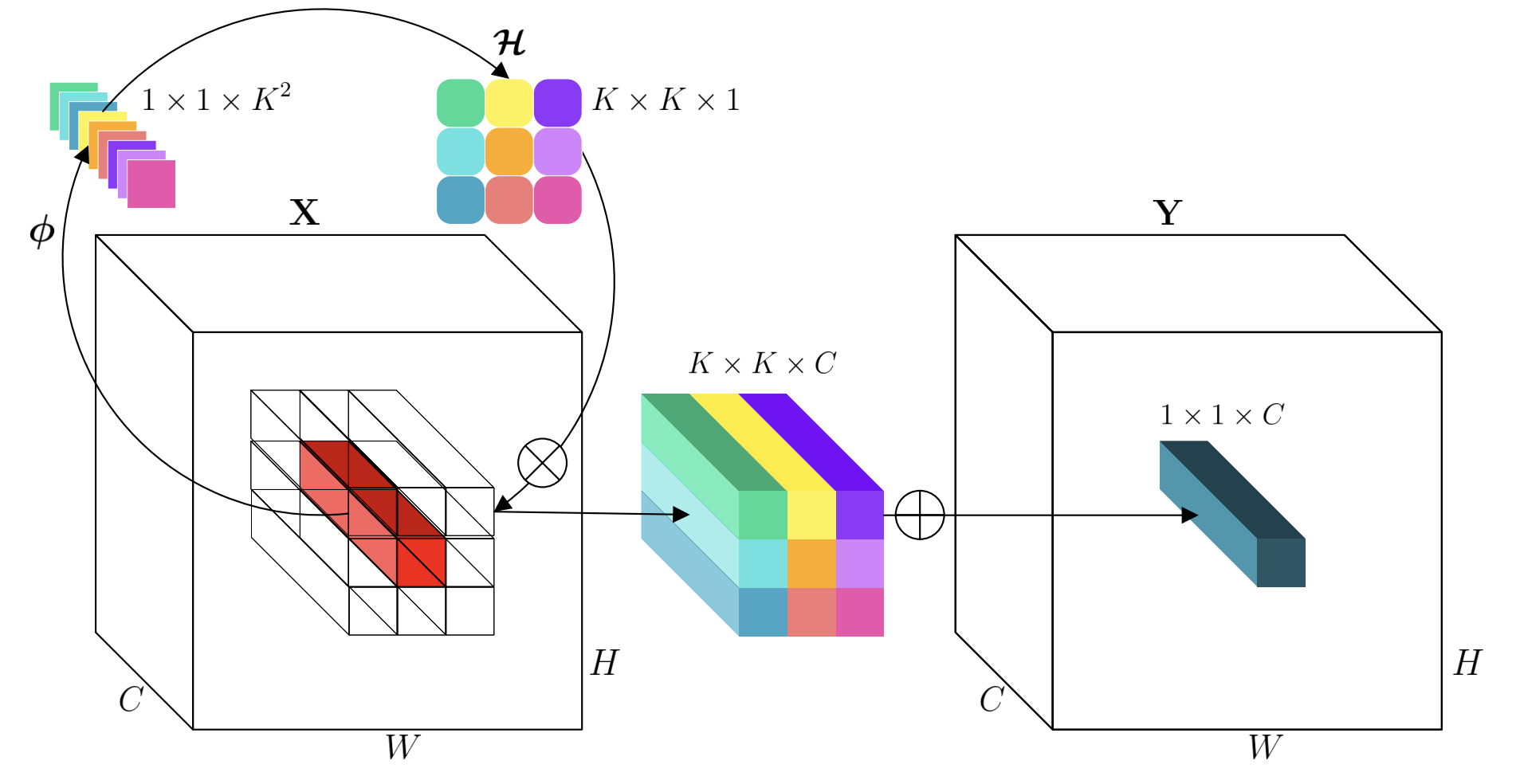 The author understands it as follows:
Involution generates kernels based on single-position channel
information, so the kernel parameters themselves already encode channel
characteristics. Through channel sharing, it avoids independent channel
calculations and the aggregation of multiple channels during output,
thereby reducing computational cost.
Basic Implementation Analysis (Code)
The kernel generation function of Involution was mentioned above, which utilizes two linear transformations to generate kernel weights. How is this implemented in practice? The original paper provided the implementation code; let's observe the specific methods of both transformations from a code perspective.
First, let's look at the PyTorch-style code:
1 |
|
In the initialization section, we can see that two Conv2d functions are used, and the convolution kernel size specified in both is 1. As we know, a \(1\times 1\) convolution kernel calculation only involves the channel dimension of the data, without touching other dimensional information. In other words, this function performs a linear combination across channels corresponding to each position. Connecting this with the formulas above, these two 2D convolution functions with a kernel size of 1 are essentially the linear transformations \(W_0\) and \(W_1\) mentioned earlier. Their forms can be written as: \[ \begin{align*} &W_0:\mathbb{R}^C \mapsto \mathbb{R}^{C//r}\\ &W_1:\mathbb{R}^{C//r} \mapsto \mathbb{R}^{K\times K\times G}\\ \end{align*} \] The first transformation \(W_0\) performs dimensionality reduction to reduce the parameter count for computing the kernel; the second transformation \(W_1\) performs mapping, projecting the compressed features into the required number of weight values.
These two transformations are the core steps of kernel generation. However, up to this point, the core parameters have not yet assumed the theoretical 3D shape. Therefore, in the forward pass section, the array is reshaped. The neighborhood of the output is unfolded into columns, which are then grouped according to channels, rearranging the dimensions to obtain the desired kernel shape \((B, G, K\times K, H, W)\). Here, \(H\) and \(W\) refer to the spatial output positions, and it is finally applied across the complete channel dimension to yield the final feature map.
Of course, the above is only a brief analysis of the basic code implementation. Understanding up to this point is sufficient to adjust the operator according to project requirements.
Simple Project Application
In the author's project, the Involution operator was used to build a neural network to predict disease probability, utilizing a dataset based on patient information and clinical data manifestations as features (refer to the UCI Heart Disease Dataset). This dataset does not consist of sequential information, yet convolution can still be used to extract relational features among attributes within a local range. As mentioned earlier, the characteristics of the Involution operator allow it to retain local feature extraction capabilities across broad data spans while demanding lower computational cost, making it suitable for non-sequential datasets as well. However, because this dataset is one-dimensional, the original code cannot be directly applied, and the operator needs to be reduced in dimension.
Once the basic implementation method is understood, the logic for
dimensional reduction is straightforward: simply modify the original 2D
convolution operations to 1D convolutions. The logic of a 1D involution
operator can be referenced in the example below: 
The kernel generation operation is carried out across channels and does not have much to do with the spatial dimensionality of the data itself. It can also be generalized to higher-dimensional datasets; however, existing libraries cannot be directly invoked, and high-dimensional convolution operations must be implemented manually.
Of course, as seen in the example above, the author also modified the activation function in the operator's kernel generation step. The original code used ReLU, while the author chose Swish, which is more sensitive to small negative values. This can be selectively adjusted according to the project. If the network constructed using the involution operator does not perform as expected, you can try adjusting the activation function. In the author's project, the improvement brought by this adjustment was relatively minor.
Thoughts on Model Acceleration Schemes
An idea occurred to the author while completing another course on parallel computing: since kernel generation in involution is computed based on fixed data, it could potentially be parallelized for acceleration. In fact, a CUDA-accelerated version is already provided in the original authors' source code. According to conventional parallelization thinking, the kernel generation operation at each position can be parallelized. The author experimented with a step-by-step parallelization method: parallelizing the matrix operations of the two convolutions separately, with a wait state at the intermediate layer. This parallelization approach achieved good speedup even when running on a CPU. However, this was merely a simple experiment, as model training is rarely conducted on CPUs in most scenarios. Perhaps there are other approaches...
References
[2] Involution: Spatial Non-sharing? A High-Performance Operator Fully Replacing Convolution | CVPR 2021