Involution的基本实现方式(学习记录)

  Involution是由Li等人于2021年所提出的新型神经网络算子。该算子的基于卷积(Convolution)设计而来，具有和卷积算子所相反的基本特征，故得名反卷积特征算子，也被称作内卷、合卷。下面统称内卷。   在笔者的本科毕业设计中，针对该内卷算子进行了学习，根据设计需要修改了算子的部分结构，并基于它设计了一个神经网络架构。本文用于粗略记录学习过程和个人理解，以及设计过程中的实现方式。笔者也初步尝试对算子进行并行化，用于学习算法和模型加速。

写在前面

本文涉及的技术论文作者目前因学术不端存在一定争议，但该篇论文本身当前没有被证实涉及争议内容。本文仅用作学习和记录，如果后续该篇论文或其技术被证明涉嫌学术问题，本文将永久归档或删除。

初步介绍

在机器学习中，卷积(Convolution)是非常经典的算法之一，特别是在计算机视觉(CV)领域。我们可以简单回顾一下二维卷积的操作，通过一个核(Kernel)，对二维特征进行滑动提取特征。在深入了解Involution之前，我们需要理解传统卷积的一些特性。卷积操作通过共享的卷积核在空间位置上滑动，这种设计具有两个核心特征：空间不变性(spatial-agnostic)和通道特异性(channel-specific)。

空间不变性意味着同一个卷积核会应用到特征图的所有空间位置，无论位置在哪里，使用的权重都是相同的。这种设计在参数使用上效率较高，但也限制了模型对不同空间位置自适应建模的能力。通道特异性则体现在卷积会为每个输出通道学习独立的卷积核，这给卷积核带来冗余。

Involution算子则是基于与卷积相反的特性而设计的，它具有空间特异性(spatial-specific)和通道不变性(channel-agnostic)。这意味着Involution会为每个空间位置生成专属的核，这些核在通道维度上共享，并具有下面的优势:

1. 自适应性增强：每个像素位置都有自己的处理核，能够更好地捕捉局部上下文信息;
2. 参数效率提升：通道共享机制大幅减少了参数量，特别是在高通道数的深层网络中;
3. 长距离依赖建模：通过增大核尺寸，Involution可以高效地建模远距离的空间关系，同时减少近距离信息丢失，平衡了远近规模的数据提取能力。

简单来说，这个算子在每个位置上生产自适应核，而通道中则通过分组确定哪些通道共用一个核心。这样就能每个元素使用不同核的同时，避免不同通道产生的冗余。接下来笔者会简单解释其原理。

原理概述

以二维数据为例，对于输入特征图 ，Involution在位置 的输出可以表示为：

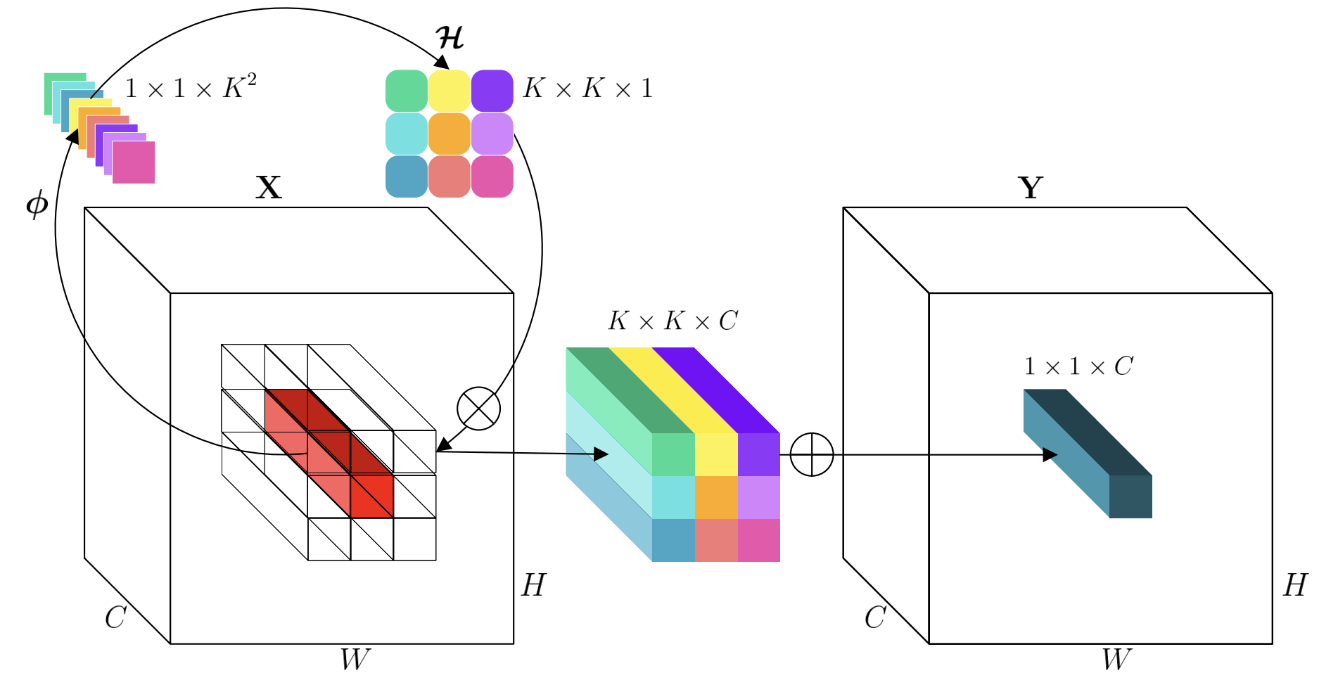其中 是以为中心的邻域， 是该位置的involution核，其核映射函数被定义为: 该式的表意是以通道作为维度的核映射为核大小乘以组别的三维度形式，可以理解为核映射操作是基于元素位置对应的通道向量进行的。下面这个函数是其具体的表达： 其中，与为两次线性变换，指激活函数。通过上述映射获得核参数后，再应用到原数据中完成核运算。下面是原论文所使用的示意图： 笔者这样理解：Involution基于单位置通道信息生成核，这样核参数本身就包含有通道特征，再通过通道共享，这样就能避免通道独立运算和输出时综合多通道的计算过程，从而减少计算量。

基本实现分析(程序)

上文提到了Involution的核生成函数，其使用两次线性变换来实现核权重的生成，那么具体怎么做呢？原论文中给出了实现的代码，尝试从代码的角度，分别观察两次变换的具体方法。

先来看看Pytorch风格的代码:

1
2
3
4
5
6
7
8
9
10
11
12
13
14
15
16
17
18

# B: batch size, H: height, W: width
# C: channel number, G: group number
# K: kernel size, s: stride, r: reduction ratio
################### initialization ###################
o = nn.AvgPool2d(s, s) if s > 1 else nn.Identity()
reduce = nn.Conv2d(C, C//r, 1)
span = nn.Conv2d(C//r, K*K*G, 1)
unfold = nn.Unfold(K, dilation, padding, s) #提取位置领域展开为列，便于后续与核参数之间的计算
#################### forward pass ####################
x_unfolded = unfold(x) # B,CxKxK,HxW
x_unfolded = x_unfolded.view(B, G, C//G, K*K, H, W)
# kernel generation, Eqn.(6)
kernel = span(reduce(o(x))) # B,KxKxG,H,W
kernel = kernel.view(B, G, K*K, H, W).unsqueeze(2)
# Multiply-Add operation, Eqn.(4)
out = mul(kernel, x_unfolded).sum(dim=3) # B,G,C/G,H,W
out = out.view(B, C, H, W)
return out

在initialization的部分中，可以看到使用了两个Conv2d函数，切函数中规定的卷积核大小均为1。我们知道，的卷积核计算实际上是只涉及数据的通道维度，而不涉及其它维度信息的。换言之，这个函数是在对每个位置所对应的通道进行线性组合。结合上文的公式推断，这两个核大小参数为1的二维卷积函数，其实就是上文提到的线性变换与，它们的形式可以写成： 第一次变换所完成的是降维，用于减少计算核参数量；第二次变换实现的是映射，将压缩后的特征映射为所需数量的权重值。

上述的两次变换是核生成的核心步骤，不过目前为止核心参数还没有体现为理论的三维形状，因此在forward pass部分中，将数组进行了reshape。将输出的领域拼接成列，然后把列按照通道进行分组，重排维度以获得理想的核形状。这里的和指的是输出的位置信息，最后将其应用到完整的通道维度，得到最后的特征图。

当然，上面只是简单地分析基本的代码实现，了解到这一步，其实也能够根据项目的需求对算子进行调整了。

简单的项目应用

在笔者的项目中，使用Involution算子构建神经网络来预测患病概率，使用的是基于患者信息和临床数据表现作为特征的数据集(参考UCI心脏病数据集)。该数据集并非序列信息，但是可以通过卷积提取范围内属性的关联特征，而上文也提到，Involution算子的特性使其可以在大跨度数据中保留局部特征提取的能力，同时会有更少的计算量，因此也可以在非序列数据集中使用。不过，因为该数据集是一维的，所以不能直接使用原代码，需要对算子进行降维。

只要了解其基本的实现方法，降维的逻辑并不难，将原先的二维卷积操作修改为一维卷积即可。一维的involution算子逻辑可以参考下面的样例：

核生成的操作是基于通道进行的，与其数据本身的维度其实没有太多关联。对于高维数据集也可以推广，只是不能直接调用现有库了，需要自己实现高维的卷积操作。

当然，上面的样例中可以看到，笔者也修改了算子核生成步骤中的激活函数。原代码中使用的是ReLU，而笔者选择了能够对小负值更敏感的Swish。这里其实可以根据项目选择性调整，如果感觉involution算子所构建的网络表现不及预期，可以尝试调整激活函数。笔者的项目中，该项调整带来的提升比较小。

模型加速方案思考

笔者在完成另一项并行计算课程时的一个想法，既然involution的核生成是基于固定数据进行计算，那么它也可能进行并行加速。实际上，在论文作者的源代码中也已经给出了一个CUDA加速的版本。根据常规的并行化思路，可以将每一个位置的核生成操作并行。笔者尝试过分步并行方法，即两次卷积分别并行化矩阵运算，然后中间层进行等待。这种并行思路在CPU上运行时也能有较好的加速效果。不过这只是一次简单的尝试，毕竟大部分情况下也不会在CPU上进行模型训练。也许能有其它思路......

参考文档

[1]Li D, Hu J, Wang C, et al. Involution: Inverting the inherence of convolution for visual recognition[C]//Proceedings of the IEEE/CVF conference on computer vision and pattern recognition. 2021: 12321-12330.

[2]Involution：空间不共享？可完全替代卷积的高性能算子 | CVPR 2021